Practical ML Dive - How to customize a Vision Transformer on your own data

Greg Schoeninger

Dec 14, 2023

Welcome to Practical ML Dives, a series spin off of Arxiv Dives.

In Arxiv Dives, we cover state of the art research papers, and dive into the gnitty gritty details of how AI models work. From the math to the data to the model architecture, we cover it all.

Practical ML Dives is meant to be a compliment to the paper deep dives. We will be taking the models we read about on Fridays, and implementing them in live running code on Wednesdays. Hopefully this cements the concepts in our brains, and sparks ideas of what we can practically build with the technology as it stands today.

If you would like to join the discussion live, sign up here. Every week there are great minds from companies like Amazon Alexa, Google, Meta, MIT, NVIDIA, Stability.ai, Tesla, and many more.

The following are the notes from the live session. Feel free to watch the video and follow along for the full context.

Previously on Arxiv Dives

The last two weeks of Arxiv Dives we covered a few state of the art computer vision techniques: Vision Transformers and CLIP.

If you missed them, find the recaps here:

Both models are applied to the image classification task, and have different strengths and weaknesses. This week we are going to give you the code to run the models, compare the models strengths, and see how they actually perform in the real world.

The Code

Let’s start by giving you a taste of what we will be building. All the code will be available here:

You can download models we train in this tutorial from this Oxen repository

Real Time Emotion Detection From Video

To give you a preview of what we will be building, take a peek at the gif below.

By the end of this dive, you will have running code for classifying video in real time into 7 different emotional categories in real time.

Use Cases

To spark your imagination, I can think of a few use cases for emotion recognition from video.

Automatic YouTube thumbnail generation, when is the person most "happy"?
Find the best frame in a live photo burst (iPhone feature)
Fan Cam at a sports area, find the most shocked person and zoom into them
Robot teacher, change tone if student get visibly angry

As we go through this example, I challenge you to think of other use cases not other for Emotion detection, but other image classification tasks.

Picking a Model

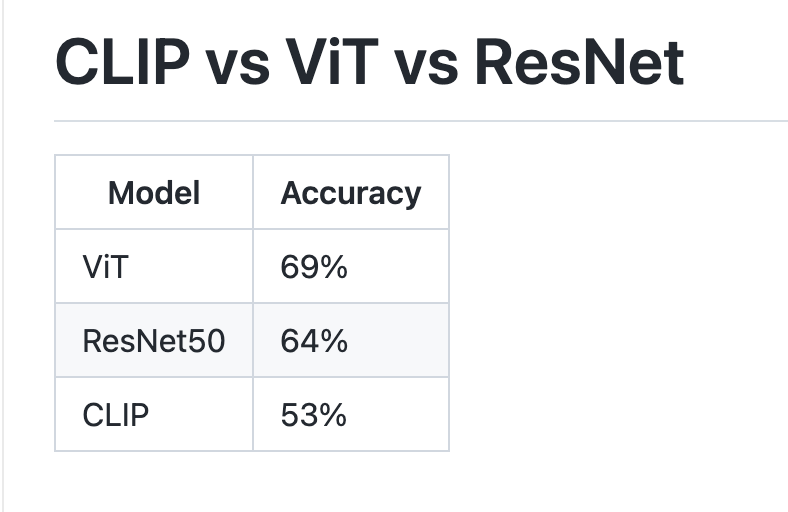
Before flushing out this tutorial, I benchmarked Vision Transformers vs a ResNet50 and Zero-shot CLIP to see which performed best.

~ TLDR ~ ViT worked the best on this task, given the data

You can explore the results for each model at the following links.

Development Environment Setup

Create a new virtual python environment as to not step on the toes of your other projects.

# Create virtual environment
python -m venv ~/.venv_practical_dives_vit

# Activate virtual environment
source ~/.venv_practical_dives_vit/bin/activate

Install the libraries we need:

pip install -r requirements.txt

You can find all the requirements here:

Where to start?

Now that we know our end goal, let’s think about the models we saw last week and think about how we can apply them to solve this problem.

Starting with the Vision Transformer, Google release the model weights for their ViT from the paper “An Image is Worth 16x16 Words: Transformers for Image Recognition at Scale”.

This model was pre-trained on ImageNet-21k which consists of 14 million images and 21,843 classes. It was then further fine tuned down to 1,000 of the top classes.

Running this model only takes about ~12 lines of actual python code.

from transformers import ViTImageProcessor, ViTForImageClassification
from PIL import Image
import sys

# Read in the file from the command line
filename = sys.argv[1]
image = Image.open(filename).convert("RGB")

# Load the image processor
processor = ViTImageProcessor.from_pretrained('google/vit-base-patch16-224')

# Load the model
model = ViTForImageClassification.from_pretrained('google/vit-base-patch16-224')

# Process the input PIL.Image into a tensor
inputs = processor(images=image, return_tensors="pt")

# Run the model on the image
outputs = model(**inputs)

# Get the logits (proxy for probability)
logits = outputs.logits

# model predicts one of the 1000 ImageNet classes
predicted_class_idx = logits.argmax(-1).item()
probs = logits.softmax(dim=1)

class_label = model.config.id2label[predicted_class_idx]
probability = probs[0][predicted_class_idx].item()

# Print the predicted class
print("Predicted class:", class_label)
print("Predicted probability:", probability)

Run live on your Web Cam

Let’s wrap this code in a loop to watch it run real time on your webcam.

from transformers import ViTForImageClassification, ViTImageProcessor
import cv2 
from PIL import Image

# Define the model_name you want to grab from hugging face
# https://huggingface.co/google/vit-base-patch16-224
model_name = 'google/vit-base-patch16-224'

# Load the image processor
processor = ViTImageProcessor.from_pretrained(model_name)

# Load the model
model = ViTForImageClassification.from_pretrained(model_name)

# Instantiate the video capture from the webcam
cap = cv2.VideoCapture(0) 

while(True): 

    # Capture frames in the video
    ret, frame = cap.read() 
		# Make sure we got a valid frame
    if not ret:
        print("Could not read frame")
        break

    # Convert from cv2.Mat to PIL.Image
    image = Image.fromarray(frame)  

    # Convert the PIL.Image into a pytorch tensor
    inputs = processor(images=image, return_tensors="pt")

    # Run the model on the image
    outputs = model(**inputs)

    # Get the logits (proxy for probability)
    logits = outputs.logits

    # model predicts one of the 1000 ImageNet classes
    predicted_class_idx = logits.argmax(-1).item()

    # Print the predicted class
    prediction = model.config.id2label[predicted_class_idx]
    print("Predicted class:", prediction)

    # describe the type of font 
    # to be used. 
    font = cv2.FONT_HERSHEY_SIMPLEX 

    # Use putText() method for 
    # inserting text on video 
    cv2.putText(frame,  
                prediction,
                (50, 50),  
                font, 1,  
                (0, 255, 255),  
                2,  
                cv2.LINE_4) 

    # Display the resulting frame 
    cv2.imshow('video', frame) 

    # creating 'q' as the quit  
    # button for the video 
    if cv2.waitKey(1) & 0xFF == ord('q'): 
        break

# release the cap object 
cap.release() 
# close all windows 
cv2.destroyAllWindows()

The problem is, we are limited to the 1,000 classes that Google trained the model on. You can see that it is getting confused by a lot going on in the image and trying to pick between 1,000 classes is pretty hard.

You can see in the image below that it classified this current frame as crash helmet which clearly is not correct. Granted - there are many objects it could classify in the image, I would expect a "state of the art" model trained on image net to do better.

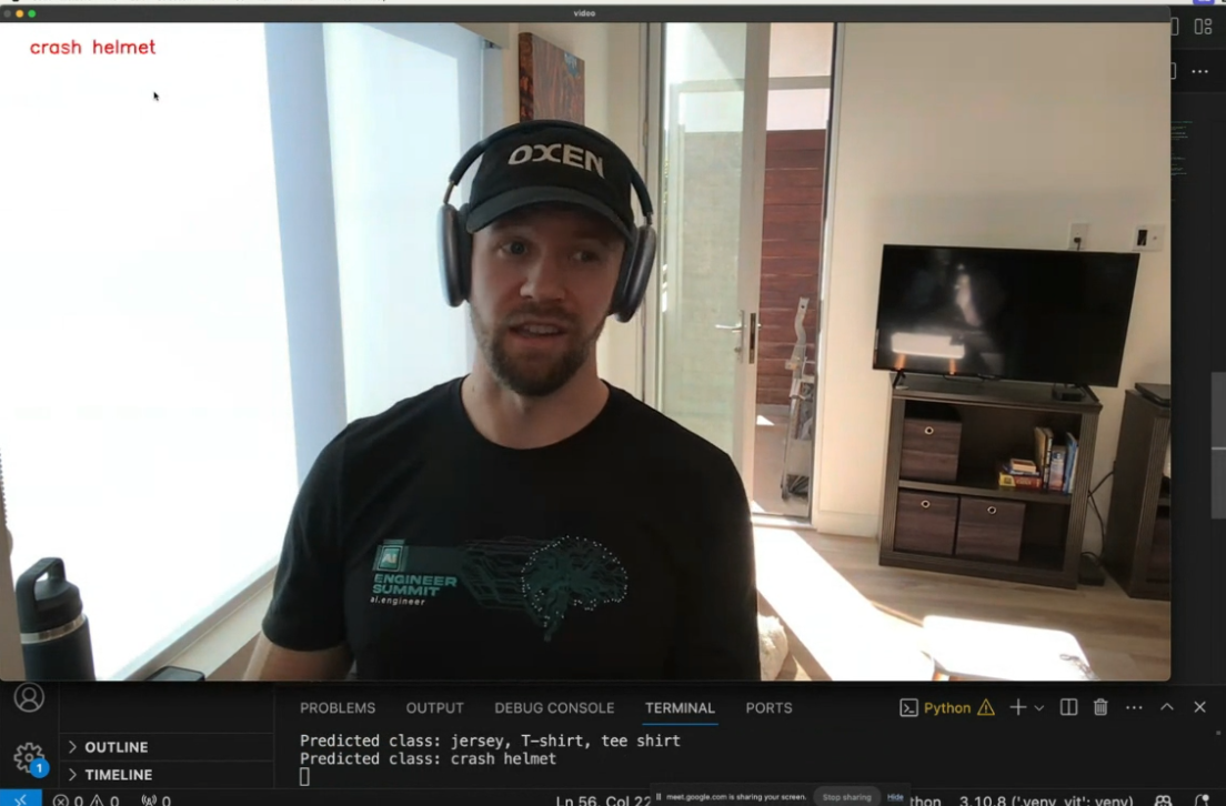
Not only is it hard to pin this image down to one class, human emotions are not captured these pre-defined set of categories. They are more animals and objects like “cat”, “dog”, “television”, etc…

We will need to train our own model to narrow the scope and be able to capture the nuance of human emotions → “happy”, “sad”, etc…

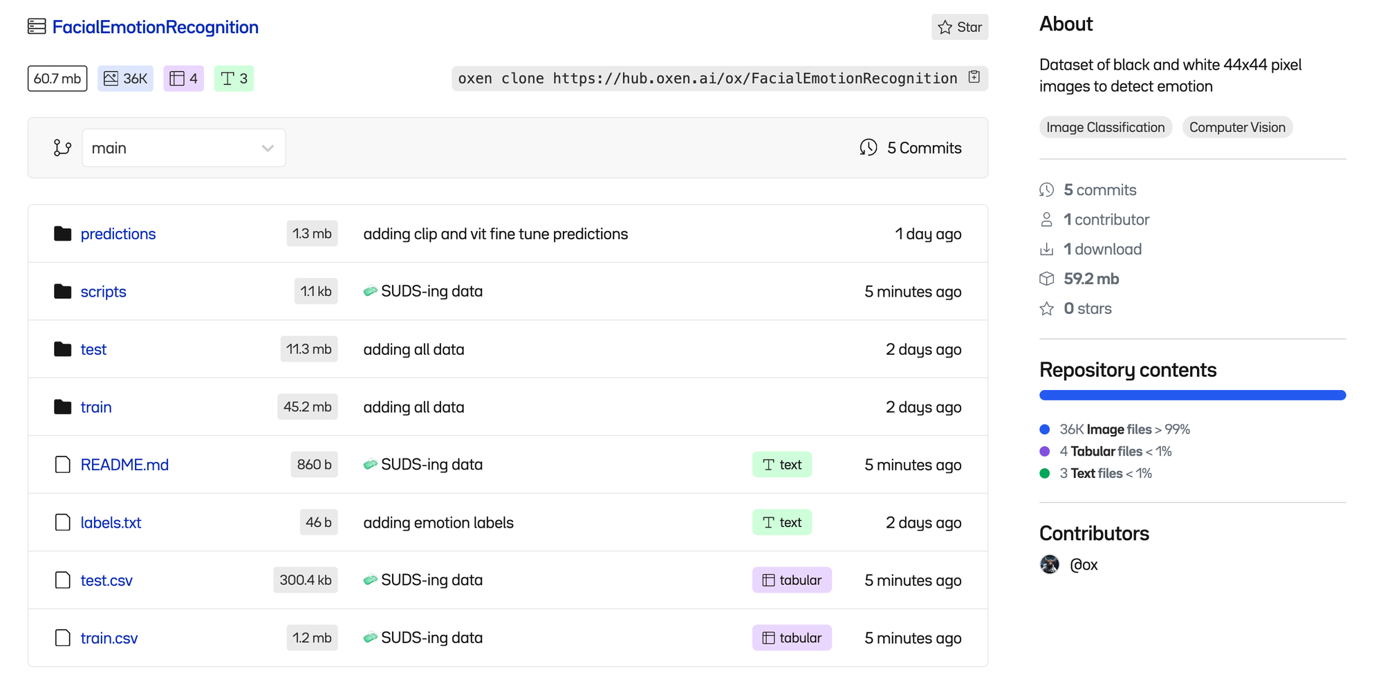
Emotions Dataset

Luckily there is already a dataset out there of images labeled with six main emotion categories, as well as a neutral category. You can find all the data on Oxen.ai.

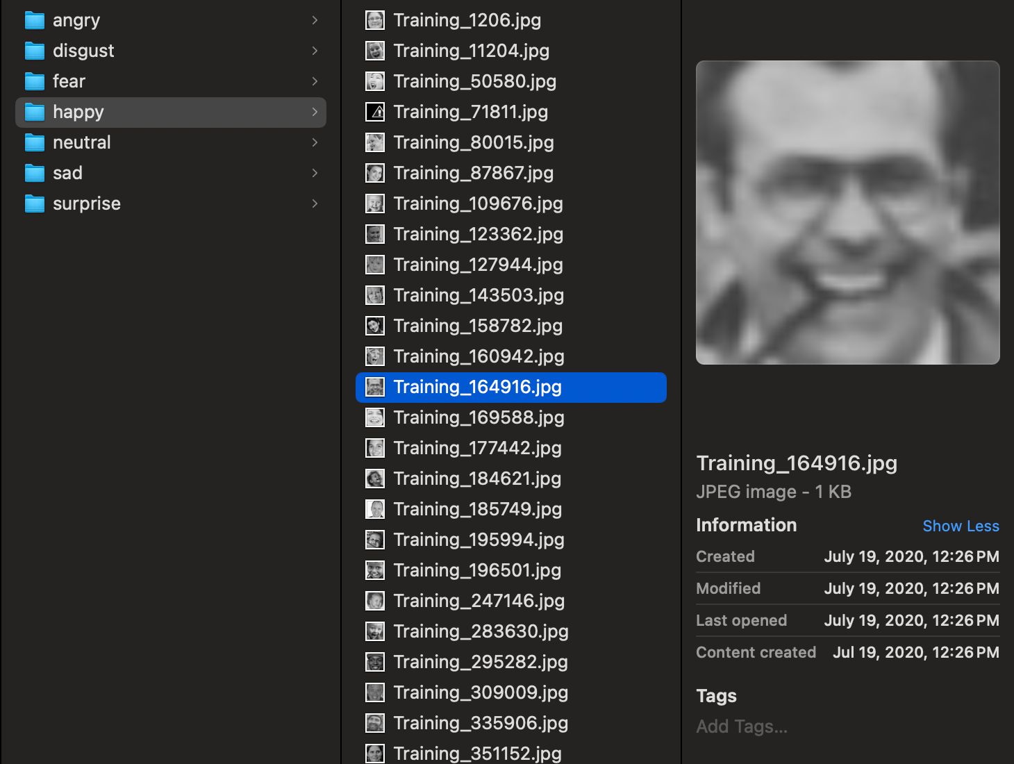
Here is a subsample of happy images from the dataset.

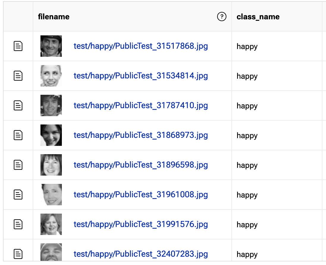
All the images in the dataset are 44x44 pixel black and white images zoomed in on the person’s face. The rest of the categories include:

Angry
Disgust
Fear
Happy
Sad
Surprise
Neutral

Explore the Dataset

The training set consists of 28,709 examples and the public test set consists of 3,589 examples. Each category within the training dataset has anywhere between 400-4000 examples.

To see some examples in the Oxen UI, follow this link, and click the train.csv file.

You can clone the entire dataset to your machine using the Oxen command line tool. If you do not have it installed, simply brew install, or follow the installation instructions for other platforms.

Install Oxen

brew tap Oxen-AI/oxen
brew install oxen

Clone the Data

Oxen can be used to quickly clone all the files to your machine so that you can explore the data locally and kick off your training.

oxen clone https://hub.oxen.ai/ox/FacialEmotionRecognition

Inspect The Data

The Oxen command line tool comes with native Data Frame processing to interact with datasets on the command line.

$ oxen df train.csv

shape: (28_709, 2)
┌───────────────────────────────────┬─────────┐
│ path                              ┆ label   │
│ ---                               ┆ ---     │
│ str                               ┆ str     │
╞═══════════════════════════════════╪═════════╡
│ train/happy/Training_50449107.jp… ┆ happy   │
│ train/happy/Training_70433018.jp… ┆ happy   │
│ train/happy/Training_85610005.jp… ┆ happy   │
│ train/happy/Training_4460748.jpg  ┆ happy   │
│ …                                 ┆ …       │
│ train/disgust/Training_81049148.… ┆ disgust │
│ train/disgust/Training_28365203.… ┆ disgust │
│ train/disgust/Training_39197750.… ┆ disgust │
│ train/disgust/Training_12525818.… ┆ disgust │
└───────────────────────────────────┴─────────┘

🧼 SUDS

We like to call this clean, re-usable data format 🧼 SUDS. It makes it easy to grok what is going on, as well as aggregate columns to get label distributions. Learn more about SUDS here.

As you can see, there are two columns in the dataset, file and label. The file column is the relative path to the file on disk. The label is which category the image falls into.

file,label
train/happy/Training_50449107.jpg,happy
train/happy/Training_70433018.jpg,happy
train/happy/Training_85610005.jpg,happy
train/happy/Training_4460748.jpg,happy
train/happy/Training_6312930.jpg,happy
train/happy/Training_25740534.jpg,happy
train/happy/Training_80076077.jpg,happy
train/happy/Training_431681.jpg,happy
train/happy/Training_76432922.jpg,happy

The images are also organized into corresponding directories by class label.

Label Distribution

We query the train.csv file to see the label distribution.

oxen df train.csv --sql 'SELECT label, COUNT(*) FROM df GROUP BY label;'

shape: (7, 2)
┌──────────┬───────┐
│ label    ┆ count │
│ ---      ┆ ---   │
│ str      ┆ u32   │
╞══════════╪═══════╡
│ angry    ┆ 3995  │
│ disgust  ┆ 436   │
│ fear     ┆ 4097  │
│ happy    ┆ 7215  │
│ neutral  ┆ 4965  │
│ sad      ┆ 4830  │
│ surprise ┆ 3171  │
└──────────┴───────┘

Looks like each class has about 3,000 or 4,000 images, except for “disgust” which only has 436 and “happy” which has 7215. This is important to keep in mind as we think about model performance. The model will perform better on classes of data it has seen more of.

Train Our Own Model

With frameworks like Hugging Face, it is not that hard to train a custom model of your own. All you need is the data, and about 200 lines of Python code. Let’s walk through how we would do it.

Let’s start with the skeleton of the command line arguments we will except and work from there.

import argparse

def main():
    # parse command line arguments
    parser = argparse.ArgumentParser(description='Train a ViT on dataset')
    parser.add_argument('-d', '--data', required=True, type=str, help='datasets to train/eval model on')
    parser.add_argument('-o', '--output', required=True, type=str, help='output file to write results to')
    parser.add_argument('-m', '--base_model', default="google/vit-base-patch16-224-in21k", type=str, help='The base model to use')
    parser.add_argument('-g', '--gpu', default=False, help='Train on the GPU if supported')
    args = parser.parse_args()

if __name__ == '__main__':
    main()

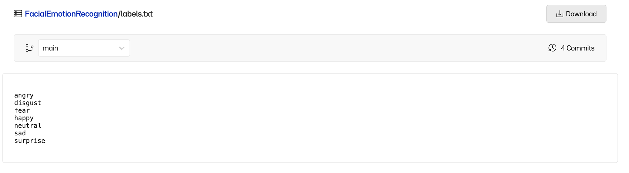
The very first thing we need to do is read in the labels we want to classify the images into. The labels can be found at the root of the dataset in labels.txt

ox/FacialEmotionRecognition/labels.txt at main

Dataset of black and white 44x44 pixel images to detect emotion. Contribute to the ox/FacialEmotionRecognition repository by creating an account on Oxen.ai

🤿 AI-Dive Library

Since the data is in a standard format, I have been working on a library to help us with these dives so we can cut to the chase of training a model, and not worry about the mundane data loading process.

I will be extending this library as we go, so that we can get to the meaty parts without having to worry about mapping files to labels, turning them into tensors, etc. You can simply pip install this library.

pip install ai-dive

This library has a LabelReader class built in that we can use to read in the class labels.

from ai.dive.data.label_reader import LabelReader

We can then use it as follows

# Parse Args
# ...
labels_file = os.path.join(args.data, "labels.txt")
label_reader = LabelReader(labels_file)
labels = label_reader.labels()
print(labels)
# ....

Load the Training Dataset

Next we have to read in the dataset and process it with the same ViTImageProcessor as before to get the data into pytorch tensors.

We have already written the data loading code for you, assuming that the data is in a 🧼 SUDS like format.

You can import our ImageFileClassificationDataset class that takes care of the heavy lifting of reading files from disk, turning them into pytorch tensors, and turning the labels into indices with our LabelReader class.

from ai.dive.data.image_file_classification import ImageFileClassificationDataset
from transformers import ViTForImageClassification, ViTImageProcessor

# Same processor as before that is tied to the model
processor = ViTImageProcessor.from_pretrained(args.base_model)

# Load the dataset into memory, and convert to a hugging face dataset
print("Preparing train dataset...")
train_file = os.path.join(args.data, "train.csv")
ds = ImageFileClassificationDataset(
	data_dir=args.data,
  file=train_file,
	label_reader=label_reader,
  img_processor=processor,
)
train_dataset = ds.to_hf_dataset()

print(train_dataset[0])
print(train_dataset[0]['pixel_values'].shape)

You can see we have a dataset object that we can now iterate over that contains a dictionary of pixel_values to label indices. In this case 3 maps to the label happy from our labels.txt file, and the images have been converted to values we can feed into our network.

{
  'pixel_values': tensor([[[
	    -0.4911, -0.4911, -0.5082,  ..., -1.4500, -1.5528, -1.6384
   ]]]),
   'labels': 3
}

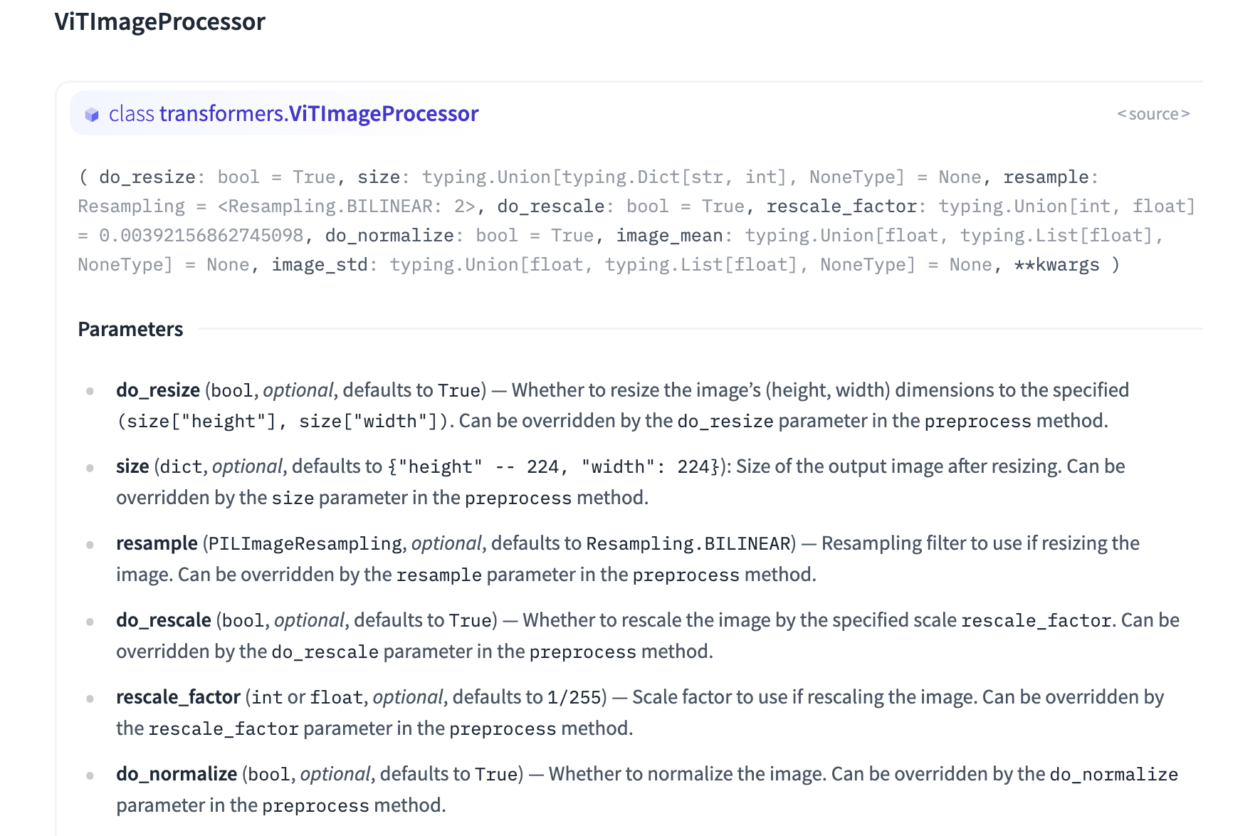
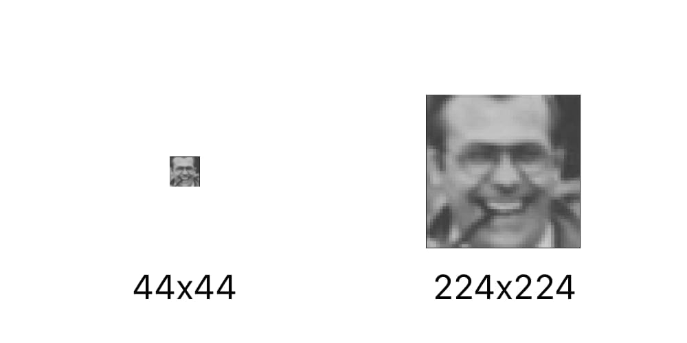
torch.Size([3, 224, 224])

If you are wondering how we went from a 44x44 pixel grayscale image to a tensor of size 3x224,224, this is all done with the ViTImageProcessor and the ImageFileClassificationDataset class.

By default this class resizes the image and resamples it using a Bilinear filter to upscale the image. Since we will be using the same VitImageProcessor for training, testing, and in the real world, everything in our pipeline should just work.

A couple important things to note on model performance, given this data loader.

Sampling up the image to 3x224x224 (150,528 data points) is way less efficient than just using the original 1x44x44 images (1,936 data points).
We could get away with a much smaller and efficient network if we wanted to train from scratch. The thing we are leveraging here is the ViT pre-training that Google has already done, so that we can fine-tune on a much smaller dataset.
If you wanted to deploy this model on the edge where you cannot run the transformers VitImageProcessor class in python code (Think an iOS app) it is very important that you use matching transforms and methods to feed the model the images.

Load the Evaluation Dataset

We also want to evaluate the model on data that it has not seen during training. We will use the test.csv file to load the evaluation dataset that we will iteratively run during training to get a sense of performance.

train_file = os.path.join(args.data, "test.csv")
ds = ImageFileClassificationDataset(
    data_dir=args.data,
    file=train_file,
    label_reader=label_reader,
    img_processor=processor
)
eval_dataset = ds.to_hf_dataset()

Load the Model

We not want to use the same ViTForImageClassification model class we used in our webcam demo, except this time we will be using our own labels. We need to pass in the mapping from our label indices to our own class names and vice versa.

model = ViTForImageClassification.from_pretrained(
    args.base_model,
    num_labels=len(labels),
    id2label={str(i): c for i, c in enumerate(labels)},
    label2id={c: str(i) for i, c in enumerate(labels)}
)

Train the Model

There are many arguments used to kick off a train, to read more about them, you can consult the documentation.

from transformers import TrainingArguments

training_args = TrainingArguments(
    output_dir=args.output, # directory to save the model
    per_device_train_batch_size=16,
    evaluation_strategy="steps",
    num_train_epochs=4, # loop through the data N times
    no_cuda=(not args.gpu), # use the GPU or not
    save_steps=1000, # save the model every N steps
    eval_steps=1000, # evaluate the model every N steps
    logging_steps=10,
    learning_rate=2e-4,
    save_total_limit=2, # only keep the last N models
    remove_unused_columns=False,
    report_to='tensorboard',
    load_best_model_at_end=True,
)

These arguments are then passed into a Trainer

from transformers import Trainer
from datasets import load_metric
import torch
import numpy as np

# We must take the dataset and stack it into pytorch tensors
# Our batch size above was 16
# So this will be a stack of 16 images into a tensor
def collate_fn(batch):
    return {
        'pixel_values': torch.stack([x['pixel_values'] for x in batch]),
        'labels': torch.tensor([x['labels'] for x in batch])
    }

# We want to evaluate accuracy of the model on the test/eval set
metric = load_metric("accuracy")
def compute_metrics(p):
    return metric.compute(predictions=np.argmax(p.predictions, axis=1), references=p.label_ids)

# Instantiate a trainer with all the components we have built so far
trainer = Trainer(
    model=model,
    args=training_args,
    data_collator=collate_fn,
    compute_metrics=compute_metrics,
    train_dataset=train_dataset,
    eval_dataset=eval_dataset,
    tokenizer=processor,
)

# Kick off the train
print("Training model...")
train_results = trainer.train()

Our computer will start chugging through all the data and training our model. To see how the training is doing over time, you can fire up tensorboard.

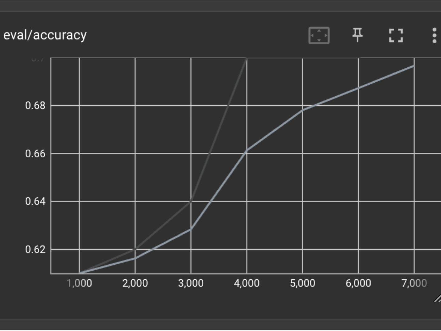
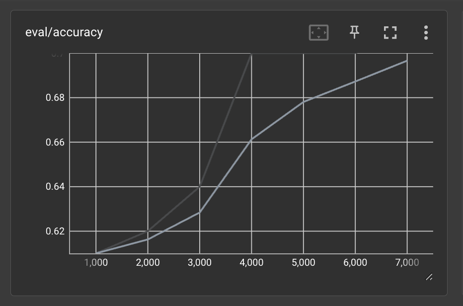
tensorboard --logdir /path/to/output_dir

Below are the loss and accuracy curves from our full training run. These curves lead me to believe that we might have been able to get higher performance if we trained even longer. We only trained for 4 epochs or full iterations through the training dataset.

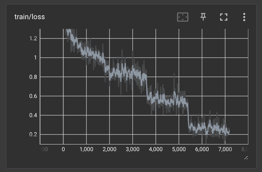
You can see the accuracy was steadily increasing as well when we stopped training.

Total Training Time

Depending on the time of day, go get some coffee ☕️ or a good nights sleep 😴 while the model trains.

This code will run on a Macbook Pro with an M1 chip at ~4.5 sec/iteration, meaning it is seeing one batch of data every 4.5 seconds. Our training batch size was 16 above, meaning we are seeing just under 4 images a second. If you remember our dataset size above, it was 28,709 images. If we see 4 per second at 60 seconds in a minute and 60 minutes in an hour that is 28709/4/60/60 ~= 2hrs to see all the training data one time. We set num_train_epochs to 4, meaning this full train will take ~8 hours to complete.

I also tried the same code on a NVIDIA RTX 3070 Ti GPU for fun, and was getting 0.35 sec/iteration which is more than a 10x speed up. Meaning the training would take about an hour to complete.

Although it is fun and “free” to train your model locally on your macbook, if you are running many experiments, it is definitely worth paying for the 1hr of compute time on a GPU, rather than waiting over night for a model to train.

Save the Model

Make sure to add these lines at the end of your script to save the trained model once the training is complete.

trainer.save_model()
trainer.log_metrics("train", train_results.metrics)
trainer.save_metrics("train", train_results.metrics)
trainer.save_state()

Using the Trained Model

Since the model can take a few hours to train, I have already trained a model on this data for you. Feel free to download it from Oxen and give it a spin.

oxen clone https://hub.oxen.ai/ox/FacialEmotionRecognitionModels

We use the same code as before to load the model, but instead of passing in the base model, we simply pass in the path to the saved model directory on our computer.

model_path = '/path/to/your/saved_model'

# Load the image processor
processor = ViTImageProcessor.from_pretrained(model_path)

# Load the model
model = ViTForImageClassification.from_pretrained(model_path)

You’ll notice that the exact webcam loop above doesn’t work that well. Remember what the training data looks like…it is a zoomed in photo of a person’s head.

Let’s crop and resize the video feed and see if that improves performance.

# ...
# Within the camera loop code above
# ...


# center crop the frame to 224x224
crop_size = 224
height, width, channels = frame.shape
left = int((width - crop_size) / 2)
top = int((height - crop_size) / 2)
right = int((width + crop_size) / 2)
bottom = int((height + crop_size) / 2)
frame = frame[top:bottom, left:right]

# flip image
frame = cv2.flip(frame, 1)

# Convert the video into PIL image
image = Image.fromarray(frame)

Saving Outputs

A great debugging and data collection technique is to save off frame by frame the predictions of the model in the wild.

import pandas as pd

# List for all the predictions
output_data = []

# Create output dir / images if it doesn't exist
images_path = "images"
if not os.path.exists(args.output):
    os.makedirs(os.path.join(args.output, images_path))

# Loop over camera
while True:
  # .. get and crop the image

  # Run the model
  prediction = model.predict(image)
  
  # Save the image to len(output_data).jpg
  relative_path = os.path.join(images_path, f"{len(output_data)}.jpg")
  full_path = os.path.join(args.output, relative_path)
  image.save(full_path)
  # Append to the output data
  prediction["file"] = relative_path
  output_data.append(prediction)
  print(prediction)

# Save the csv to the output dir
df = pd.DataFrame(output_data)
df = df[["file", "prediction", "probability", "time"]]
df.to_csv(os.path.join(args.output, "predictions.csv"), index=False)

We can now upload these outputs to Oxen.ai to debug further, label as test data, or even split up and merge into a future training dataset.

BONUS - Using CLIP without training

Remember how it took an hour to 8 hours to train the model above? What if you could get the same behavior without training?

Enter CLIP 📎

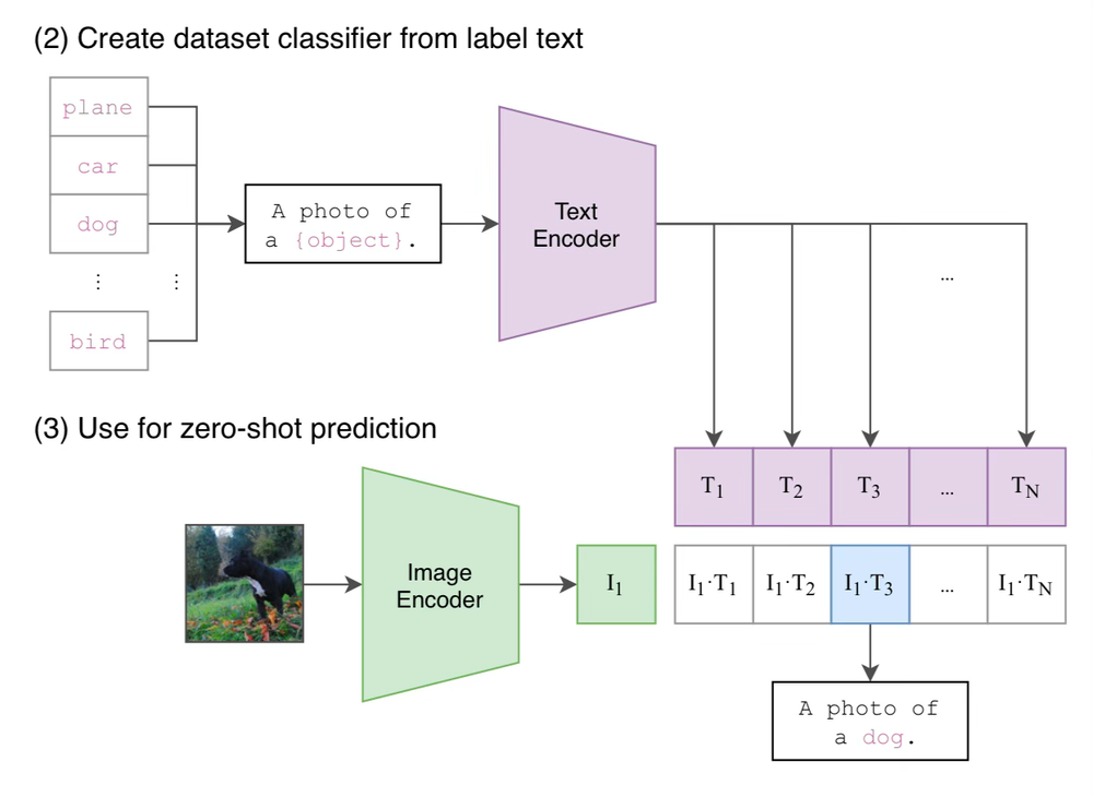
With CLIP you can dynamically define the classes when running the model to any phrase in the English language. This is what we call "zero-shot" image classification, because it did not require any training examples.

from PIL import Image
from transformers import CLIPProcessor, CLIPModel

model = CLIPModel.from_pretrained("openai/clip-vit-large-patch14")
processor = CLIPProcessor.from_pretrained("openai/clip-vit-large-patch14")

filepath = "face.jpg"
image = Image.open(filepath)

class_labels = [
  "happy",
  "sad",
  "surprised"
]
prompt = "a photo of a face that is "
prompts = [f"{prompt} {label}" for label in class_labels]
inputs = processor(text=prompts, images=image, return_tensors="pt", padding=True)

outputs = model(**inputs)

# this is the image-text similarity score
logits_per_image = outputs.logits_per_image

# we can take the softmax to get the label probabilities
probs = logits_per_image.softmax(dim=1)

# We can take argmax to get the index
predicted_label_idx = logits.argmax(-1).item()

# Get the label name
predicted_label = class_labels[predicted_label_idx]
predicted_prob = probs[predicted_label_idx]

print(f"{predicted_label}: {predicted_prob}")

Note: The per frame throughput is much slower because you have to run the language model on every phrase to compute the score of each one. The strength is, you can swap out the labels on the fly to pretty much anything in the english language without retraining.

If you remember from the stats at the top, zero-shot CLIP performed the worst out of all the metrics, but surprisingly still got over 50% accuracy on all 7 classes with no training. Random guessing would be 14% accuracy.

Conclusion

Thanks for diving in with us! The code with be posted on GitHub and the data on Oxen.ai

Next Up

Thanks for sticking around this far! To find out what paper we are covering next and join the discussion at large, checkout our Discord:

Join the oxen Discord Server!

Check out the oxen community on Discord - hang out with 269 other members and enjoy free voice and text chat.

Discord

If you enjoyed this dive, please join us next week!

All the past dives can be found on the blog.

The live sessions are posted on YouTube if you want to watch at your own leisure.

Best & Moo,

~ The herd at Oxen.ai

Who is Oxen.ai?

Oxen.ai is an open source project aimed at solving some of the challenges with iterating on and curating machine learning datasets. At its core Oxen is a lightning fast data version control tool optimized for large unstructured datasets. We are currently working on collaboration workflows to enable the high quality, curated public and private data repositories to advance the field of AI, while keeping all the data accessible and auditable.

If you would like to learn more, star us on GitHub or head to Oxen.ai and create an account.