Diffusion models have been popular for computer vision tasks. Recently models such as Sora show how you can apply Diffusion + Transformers to generate state of the art videos with impressive quality.

Is it possible to apply these techniques to text generation? If so, what would be the benefits? Today we are diving into text diffusion, and how it is an interesting research direction to replace auto regressive language models.

Resources

Discrete Diffusion Modeling by Estimating the Ratios of the Data Distribution

Despite their groundbreaking performance for many generative modeling tasks, diffusion models have fallen short on discrete data domains such as natural language. Crucially, standard diffusion models rely on the well-established theory of score matching, but efforts to generalize this to discrete structures have not yielded the same empirical gains. In this work, we bridge this gap by proposing score entropy, a novel loss that naturally extends score matching to discrete spaces, integrates seamlessly to build discrete diffusion models, and significantly boosts performance. Experimentally, we test our Score Entropy Discrete Diffusion models (SEDD) on standard language modeling tasks. For comparable model sizes, SEDD beats existing language diffusion paradigms (reducing perplexity by $25$-$75$\%) and is competitive with autoregressive models, in particular outperforming GPT-2. Furthermore, compared to autoregressive mdoels, SEDD generates faithful text without requiring distribution annealing techniques like temperature scaling (around $6$-$8\times$ better generative perplexity than un-annealed GPT-2), can trade compute and quality (similar quality with $32\times$ fewer network evaluations), and enables controllable infilling (matching nucleus sampling quality while enabling other strategies besides left to right prompting).

arXiv.orgAaron Lou

Language Modeling by Estimating the Ratios of the Data Distribution | Aaron Lou

Modern large language models (like ChatGPT) learn to generate new samples by modeling the data distribution of natural text. However, the underlying methodology has largely remained stagnant over the last century: although different architectures have been developed, models are all based on autoregressive modeling (i.e. next token prediction). In this blog post, I will talk about our work on Score Entropy Discrete Diffusion models, an alternative probablistic modeling technique that achieves highly competitive performance (at the scale of GPT-2) while introducing distinct algorithmic benefits. Our empirical results challenge the longstanding dominance of autoregressive modeling and can potentially pave the way for an alternative class of language models built from radically different principles.

Aaron LouAaron Lou

Paper Authors: Aaron Lou, Chenlin Meng, Stefano Ermon - Stanford University, Pika Labs.

Core Contribution

This paper introduces a new loss function, called score entropy, and model architecture, Score Entropy Discrete Diffusion Models (SEDD). Prior to this work, autoregressive (next-token predicting) models were miles ahead of non-autoregressive approaches like diffusion modeling.

SEDDs are the first published example of a diffusion-based model architecture showing competitive performance with best-in-class autoregressive architectures of the same model size, achieving a better perplexity score than GPT-2.

But why are we so excited about matching performance to a 2019 model?

Many researchers believe that there are inherent limitations to autoregressive modeling:

• Since generating token i is dependent on generated tokens 0 .. i-1, generation must happen sequentially, from left-to-right. This prevents useful, novel generation styles like infilling.
• Sequential sampling is slower, as its dependence prevents it from being parallelized at inference time. Generating token n requires having first generated token n-1, etc.
• Sequentially sampled outputs tend to degenerate as the sequence length increases. This can be remedied through techniques like nucleus sampling, but these introduce biases into the generation.

Probability Distributions for Generative AI

When building generative AI, we are looking to create a model which will approximate a given distribution of data as closely as possible.

That distribution could be any type of data:

• Coherent english sentences
• Bug-free, best-practice python code
• Photorealistic natural images
• Cute, pixar-like cartoons

How do we actually accomplish this? Jeremy Howard has a great explanation of the underlying mechanism in the following video.

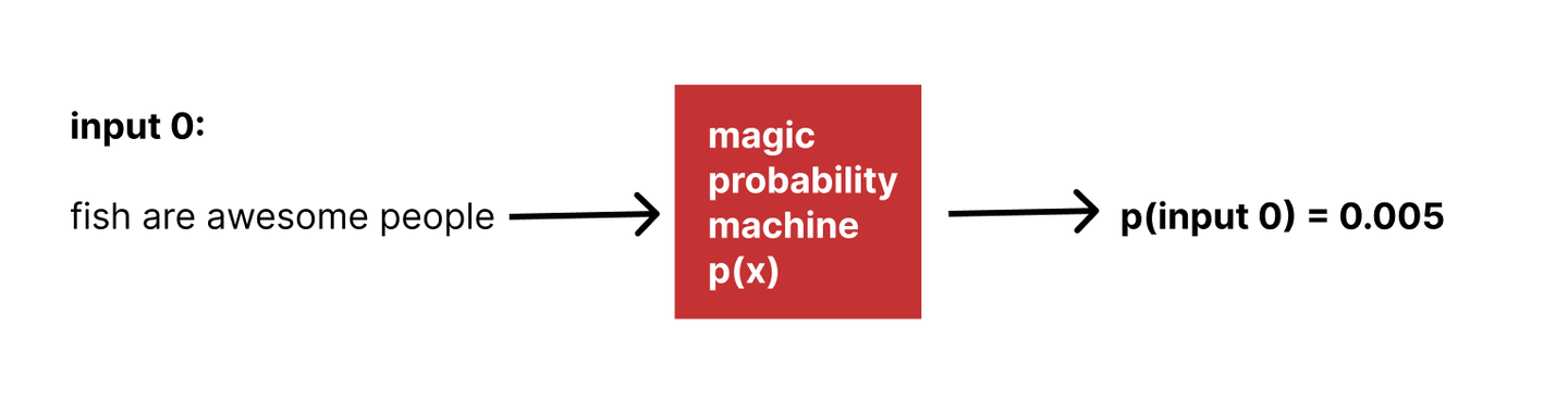
What if we had some arbitrary black box that could tell us the probability that any given input was a member of our target population?

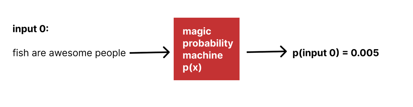
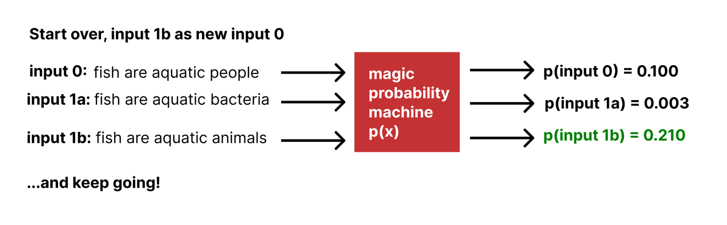
Could we use that to generate sentences which are more and more consistent with our target population? How?

We can then repeat this process with the new sentence until we get a very high-probability output—which will by definition be very well-aligned with our target population.

Yay! We've just solved generative language modeling.

(jk)

Problem #1

We don't have that black box.

Let's rename the mysterious black box above to what it is: the probability mass function of the data distribution in which we're trying to generate: p_data.

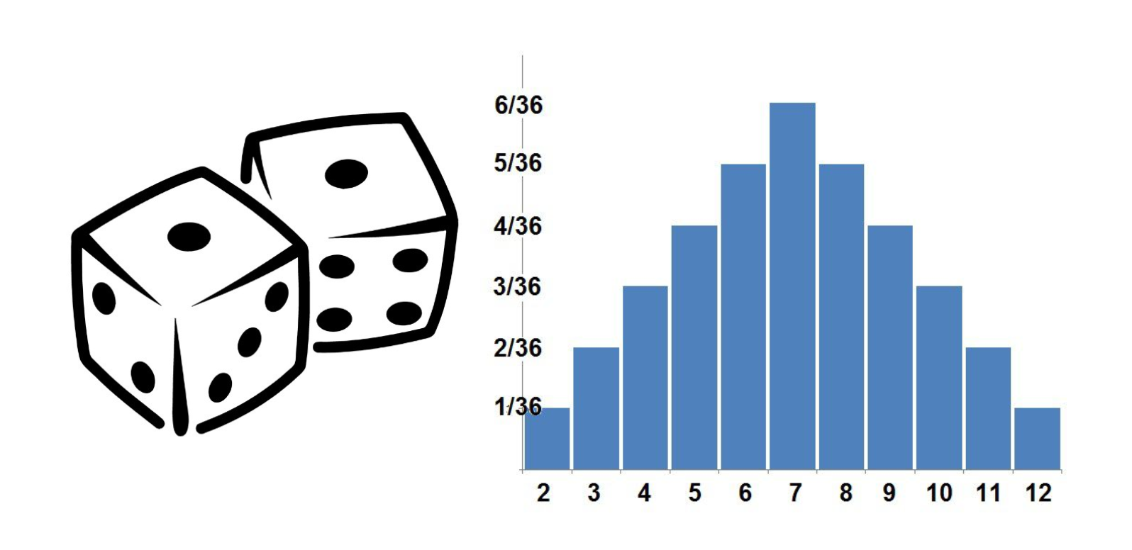
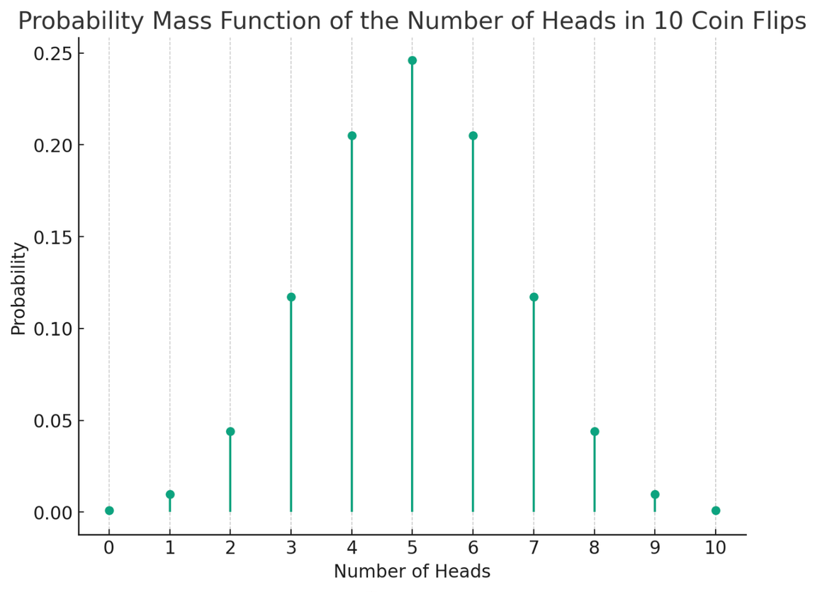
Refresher: for some distribution, its probability mass function (pmf) is a function that maps any input to the probability of an input's occurrence.

For the distribution of the number of heads in 10 coin flips, the pmf would look like this—where 5 is the most likely outcome at 24.7% probability.

But for the distribution of a real-life natural language domain like “helpful, correct english sentences,” the probability mass function is much more complicated and impossible to directly observe.

So, as deep learning practitioners, we grab our favorite hammer (large, highly parameterized deep neural networks) and get to work learning to approximate this underlying distribution.

Solution #1

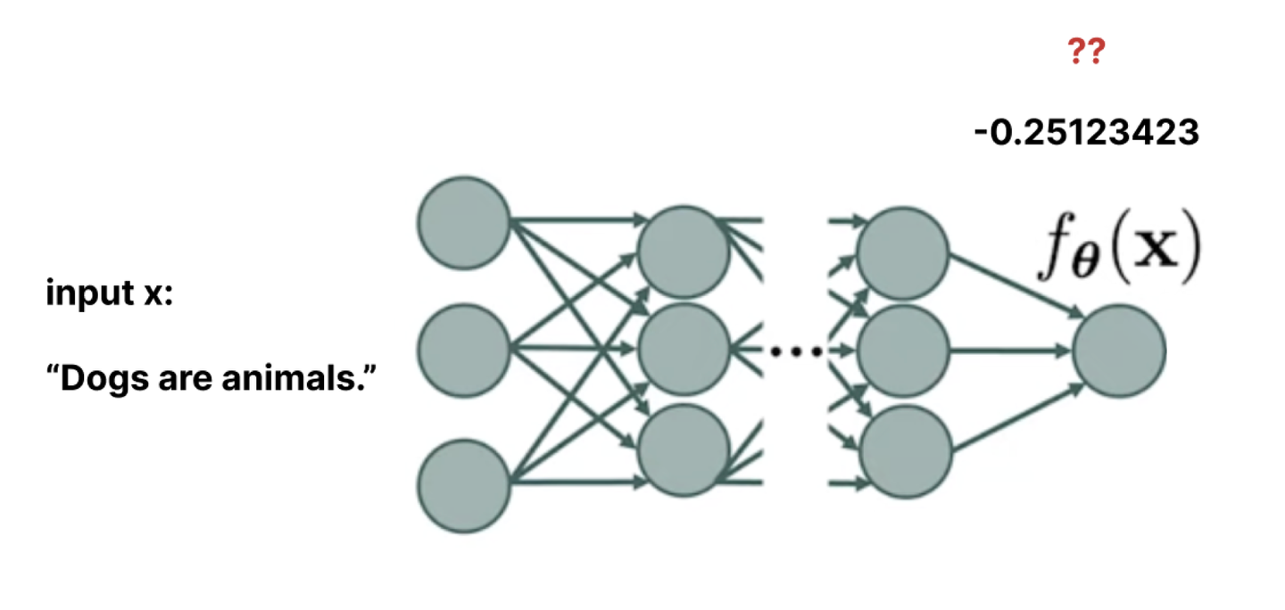
Train a neural network to approximate the probability mass function. We can instantiate a large, highly flexible neural network, feed it inputs from our data (as well as examples not from our data), and try to view the outputs as our probability mass values.

Visuals adapted from Yang Song, here.

This raises a problem, though. There are two primary constraints that must be satisfied for a function to be a probability mass function, and thus to be valid for our purpose of generating high-quality output samples.

Constraint 1: f_theta(x) must be ≥ 0 for any input x.

This makes sense, since a PMF value at x is the probability of x occurring.

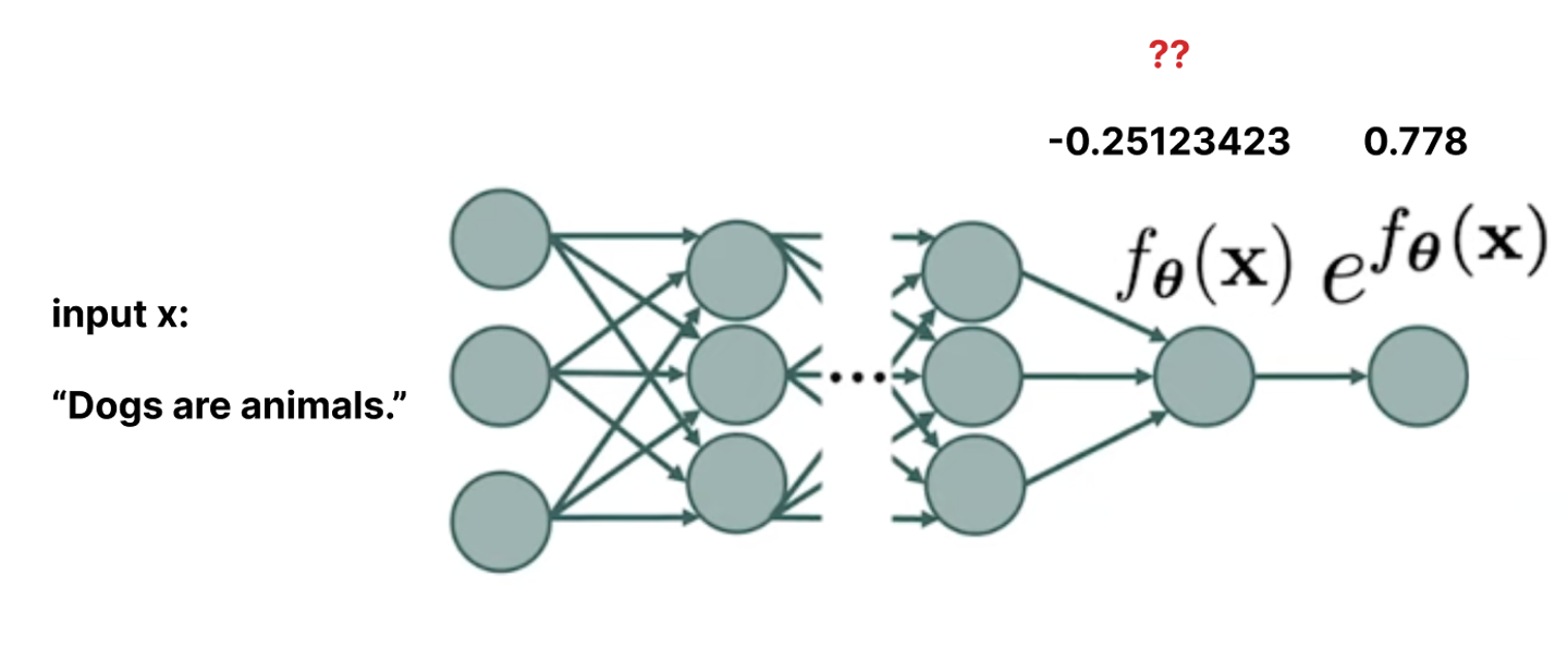
No big deal, we’ll just exponentiate all the network outputs to ensure our network outputs meet this constraint.

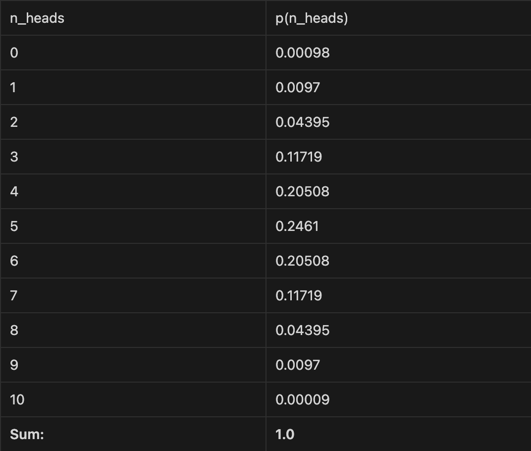
Constraint 2: The sum of f_theta(x) for all possible x must == 1.

This, again, makes sense given that we are looking to output probabilities. See the “heads in 10 flips example”.

How do we adjust our output probabilities to account for this?

Sum up the exponentiated outputs of all possible input X to get a normalizing constant, Z - then divide each value by it.

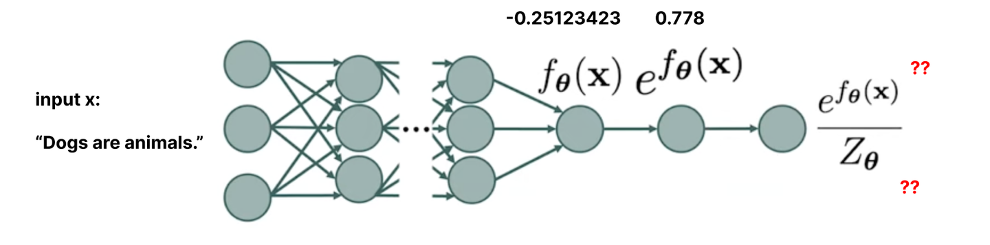
Alright - so let’s sum up the exponentiated activations of all possible inputs, and sum them up to get our Z_theta. All we have to do is feed in every possible input to the neural network, add them up, and we get our Z. Divide by that, and we’ve developed our 🐐 general model.

Problem #2

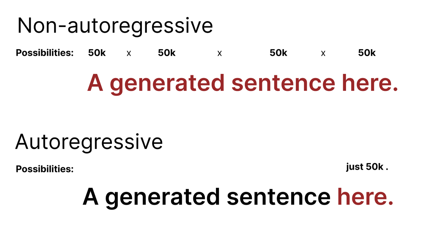
The normalizing constant, Z_theta, is intractable. The problem is with the notion of “all possible inputs” here. This set is comprised of all possible input-length sequences of valid tokens. We’ll use GPT-2 as an example here, as it’s the model size and class that these author’s match and compare against.

GPT-2, for example, has a vocabulary of 50,257 tokens. It also has an input sequence length of 1024.

Since tokens can be repeated, the size of the set we need to compute output likelihoods for here is…50,257^1024....which is more than the than the number of atoms in the known universe.

Solution #2

Predict the next word! Or in fancy terms, autoregressive modeling.

This conundrum is exactly what motivates autoregressive modeling - and why it works so well. It allows us to escape this intractability!

This reframes the probability calculation such that each token to be generated (token_i) is conditioned on all those that came before it (token_i-1 through token_0).

This means that all previous tokens are essentially fixed in time at the time of generating token i - meaning there are only number of possibilities, rather than <vocab size * context length>.

We’re looking to move beyond predicting the next word and break free of some of it’s limitations.

Solution #3:

Model score, not probability mass. Recall our earlier thought experiment.

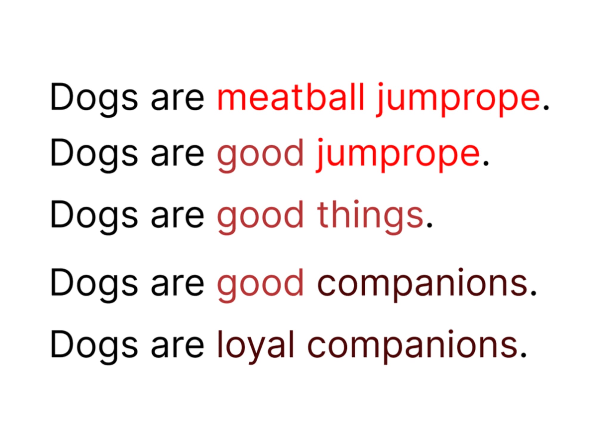
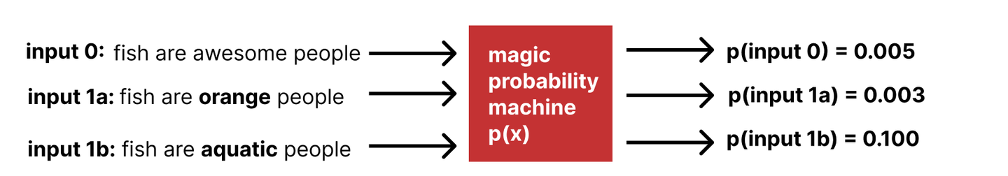
When we were taking small iterative steps in the right direction, changing one word at a time and comparing the output probabilities…how did we decide which word to swap?

We didn’t use the actual, absolute probability values — we stepped in the direction of the strongest rate of positive change in probability.

If we teach our model to learn the direction in which to move to increase the fidelity of our outputs, we can achieve our goal of generating faithful samples without needing to compute that intractable “Z” constant.

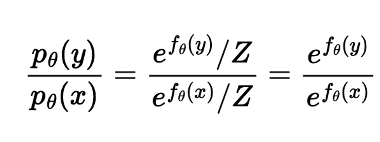
For an x in the training data, and any other random input y…How unlike our underlying data distribution is y?

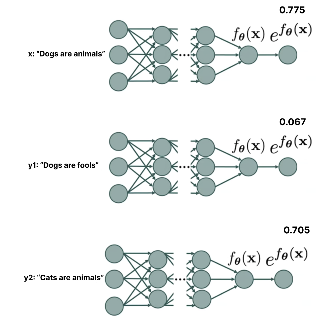
Concrete score of x with respect to y2: 0.705 / 0.775 = 0.901

Concrete score of x with respect to y1: 0.067 / 0.775 = 0.081

This ratio concrete score is now model-able by our network (in theory) since we no longer depend on an intractable constant.

The authors also restrict the set of Y which are “close” to x, defined by Hamming distance == 1.

Hamming distance is how many tokens you change in the sentence.

• Dogs chase animals ✅ (hamming = 1)
• Broccoli are vegetables ❌ (hamming = 2)
• Seven ham eighteen ❌ (hamming = 3)

Enter Diffusion

You may be looking at p(y) and p(x) and thinking we still don't have the full ground truth distributions because they are intractable. This is where the diffusion process comes in.

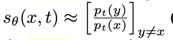
Our way out of this conundrum is to rather than attempt to estimate p(y)/p(x) directly, to estimate p_t(y) / p_x(t) perturbations of the original data distribution, for various time steps t.

Basically - we add noise to the existing data, changing it from an existing, unmeasurable distribution p(x), to a new distribution, p_t(x), which we can make assumptions about and train our network to learn, for a variety of different time steps t.

We can’t “check our work” with the unknown quantity p(x), but we can check our work on the amount of noise that we added. We know what was added, so we have the answer key.

If we can estimate the effects of the noise, we can reverse it, and our model can take us from noise to a coherent generation at inference time.

Learning the concrete score through diffusion

We’ve seen in past dives that images are gradually diffused for model training through the iterative addition of small-scale random noise across all pixel values at once. This works well to slightly noise the image without fully destroying the underlying signal.

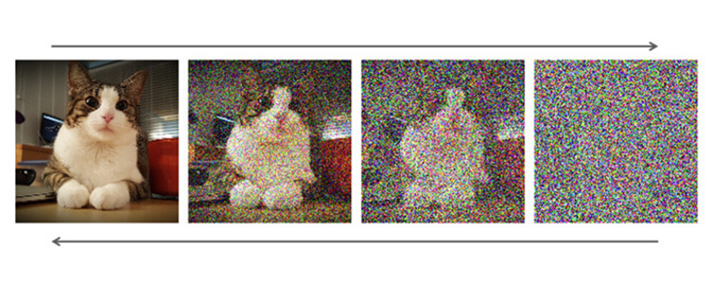
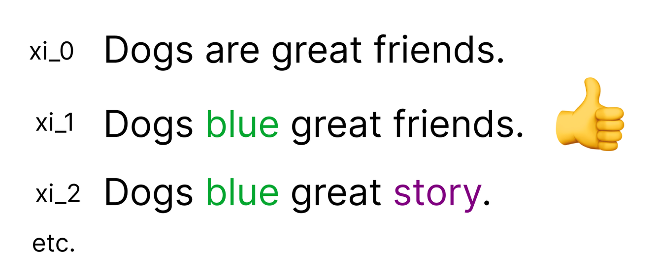
Can we do the same with text?

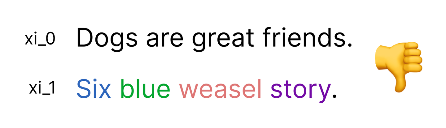
Nope - if the entire sequence is uniformly changed, the original signal is completely destroyed. We need some signal to recover for our network to be able to accurately learn what noise was added!

An excellent gif from the first author (Aaron Lou here) here illustrating this in practice:

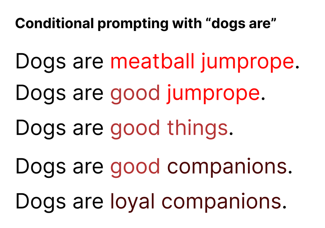
Reversing the diffusion process to generate new samples

Once we’ve learned these concrete score ratios for our diffused data, we can use them to iteratively reverse the process on new, input data.

To generate a random (unconditional) new sample:

• Start with a noised input sequence (diffusion scheduler time = maximum T)
• Using our learned concrete ratios and diffusion scheduler, step “backwards” in time, sampling what the model believes is a less and less noised version of the previous input
• Arrive at t = 0, with a “denoised” input zero which will, under a well-trained network, closely resemble the training data distribution.

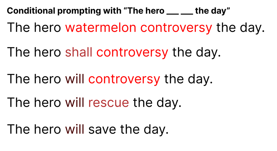
Conditioning (prompting)

Rather than starting with a fully noised sample, insert desired prompt tokens (these don’t just have to be at the beginning, as we’ll discuss 👀) and fill the rest with diffused tokens.

Apply the iterative denoising schedule only to the diffused tokens:

Evaluation

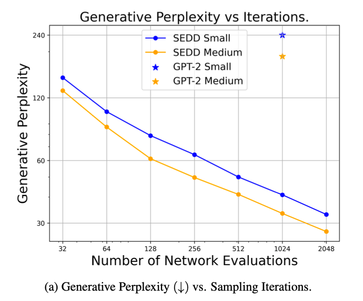
How does this model perform in comparison to existing autoregressive techniques, and what advantages does it provide over them? Perplexity evaluation on unconditional tasks (perplexity heuristic: how perplexed the model is by the generated sample - lower is better).

So what?

One more time—GPT2 is old news. why is this impressive? Several reasons!

Unlike autoregressive models (GPT-2 et. al), text diffusion models are not limited to left-to-right prompting. In particular, the approach we discussed under “conditional generation” allows for infilling, a commonly-used technique in imagery but infrequently applied to text.

Another reason is that text diffusion models in theory have better natural long-term coherence, as they are less prone to degeneration at longer sequence lengths. Autoregressive models use additional “annealing” techniques to prevent sequence degradation over time. If you mess up one word when predicting the next word, it messes up the whole sequence.

Finally, diffusion models enable a direct tradeoff of compute for sample quality.

As mentioned earlier, the diffusion process involves taking small steps backwards in the diffusion timescale, iteratively removing noise to generate higher and higher fidelity samples. This allows inference-time flexibility to determine how many denoising steps you want to take.

More steps = higher quality = more expensive.

This type of tradeoff is largely not available in autoregressive models, and allows a more efficient utilization of compute for areas where sample fidelity is less important than throughput—and vice versa.

Takeaways

I think this is a really promising direction for text diffusion modeling, and I’d love to see what it looks like scaled up! Just because these models are competitive with GPT-2 at a similar size doesn’t automatically guarantee they’ll be competitive with GPT-3, 3.5, 4 etc. class autoregressive models when scaled up—but it’s a really exciting start.

Stick with us next week as we dive into the code for this project and break it down to a simple end to end example with a character level language model.