Join the Oxen.ai "Nerd Herd"

Every Friday at Oxen.ai we host a public paper club called "Arxiv Dives" to make us smarter Oxen 🐂 🧠. These are the notes from the group session for reference. If you would like to join us live, sign up here.

The first book we are going through is Generative Deep Learning: Teaching Machines To Paint, Write, Compose, and Play.

Unfortunately, we didn't record this session, but still wanted to document it. If some of the sentences or thoughts below feel incomplete, that is because they were covered in more depth in a live walk through, and this is meant to be more of a reference for later. Please purchase the full book, or join live to get the full details.

Auto Encoders

Before we get to “variational auto encoder”, it is important to understand what an auto encoder is.

Keep in mind, this example is for images, but the same can be done for text, audio, video, or just a straight data frame itself.

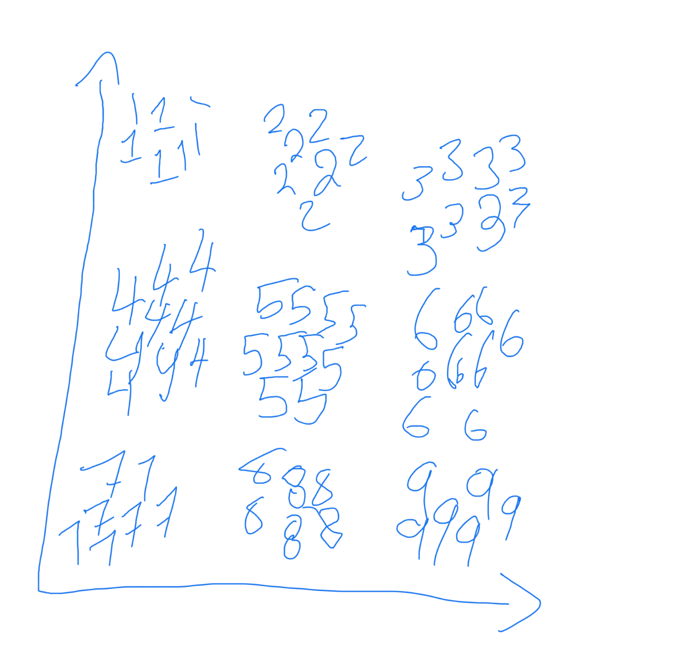
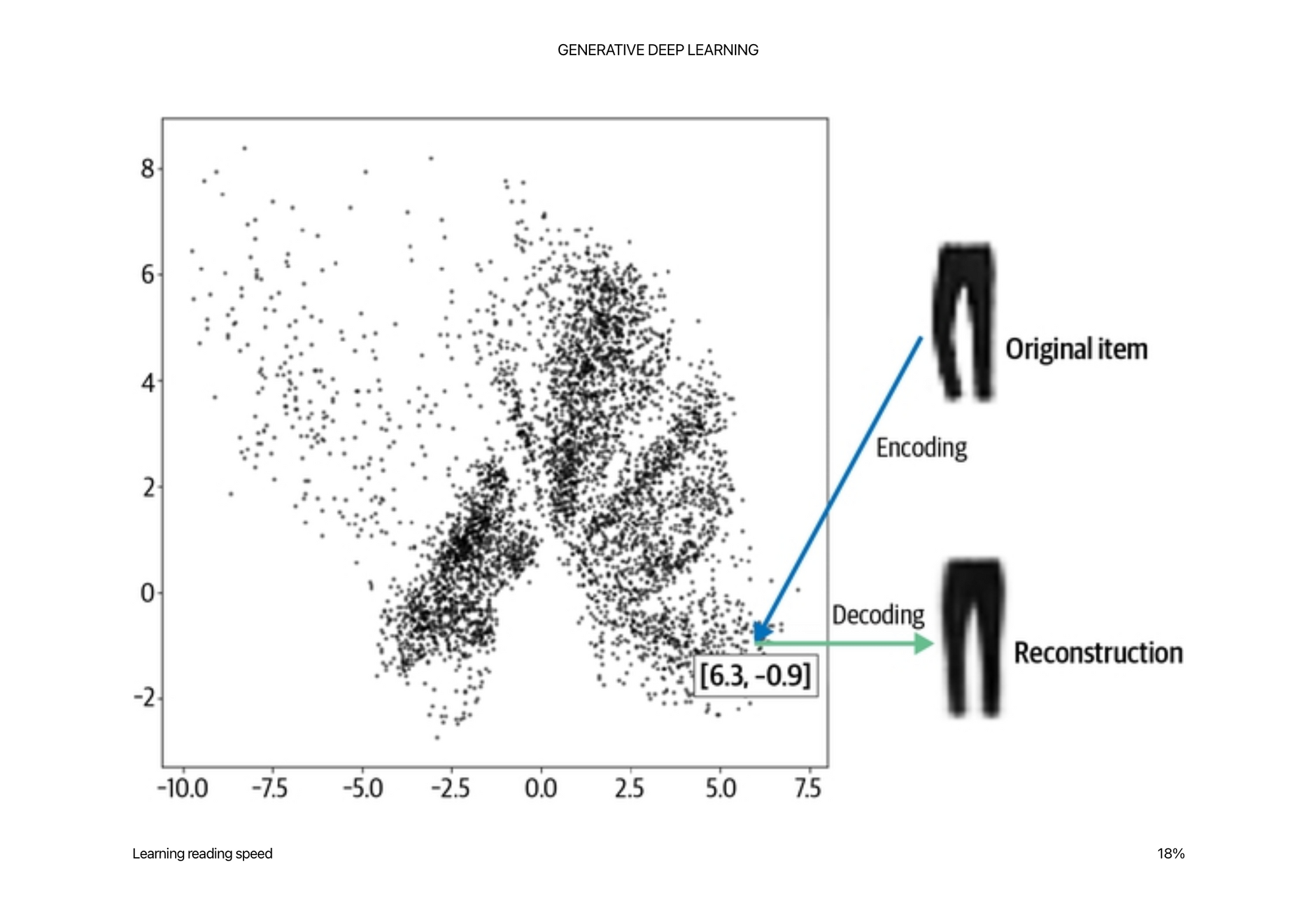
Imagine you have one person, who is the encoder, who is organizing information on a 2D wall. Then you have a second person, who is the decoder, that is trying to decode that information. If the data was digits, like mnist, the encoder might organize them in a grid where all the 1s were together in the upper left corner and all the 9s were together lower right corner. Then the encoder could simply point to a place on the wall, and the decoder would be able to draw a digit from simply the 2D information that the encoder gave them.

In this book he gives the example of “an infinite fashion closet” where the encoder puts a piece of clothing in there and then can point to a point and the decoder can generate a piece of clothing from there.

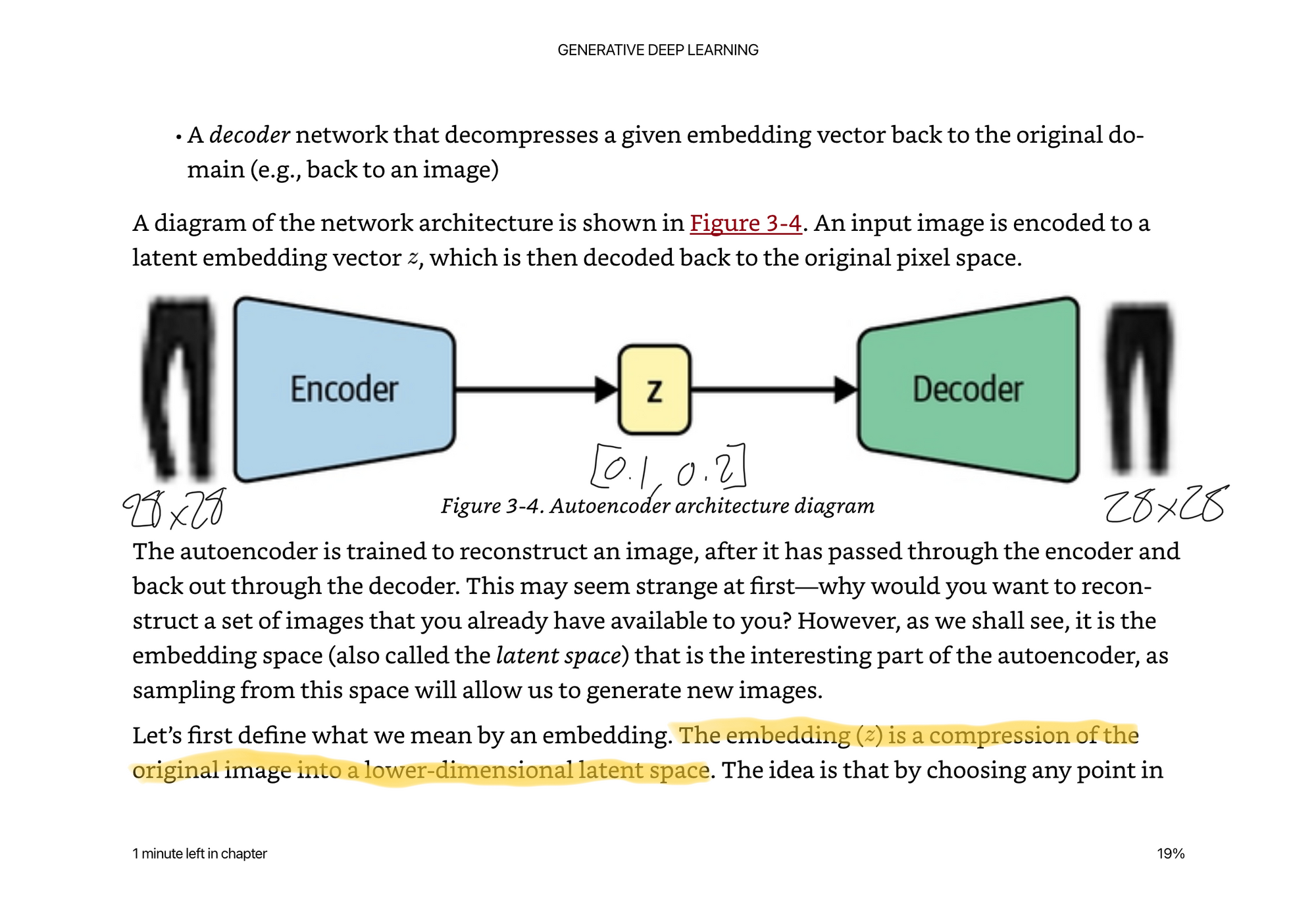
Encoder Decoder Architecture

It is the encoders job to take the 28x28 pixels and compress them, or organize them, or whatever word you want to use into a smaller dimensional space. Then it is the decoders job to take the smaller representation and blow it back up into another 28x28 image.

Usually the latent space has more than 2 dimensions, it is just easy for us to visualize 2 or 3D as humans. But like we mentioned before there are many attributes that may be helpful to encode like “has mustache” or “is tall” or “blue jeans” or whatever. These are implicitly learned, not explicitly set.

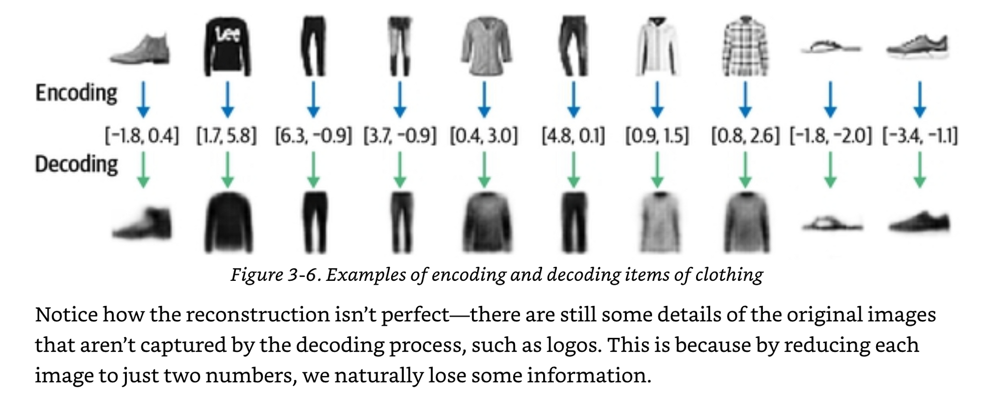
When you think about it, if you are only given two dimensions to represent what is in the image, you can only represent things like “blue jeans are over here”. The more dimensions you have the more nuance you can encode like “tattered blue jeans bell bottoms with flowers on the back left pocket”. This requires you have a ton of data representing that distribution though.

When decoding or reconstructing the image from the latent space, you need to have some metric of “how well we are doing”? This is what's called the loss function.

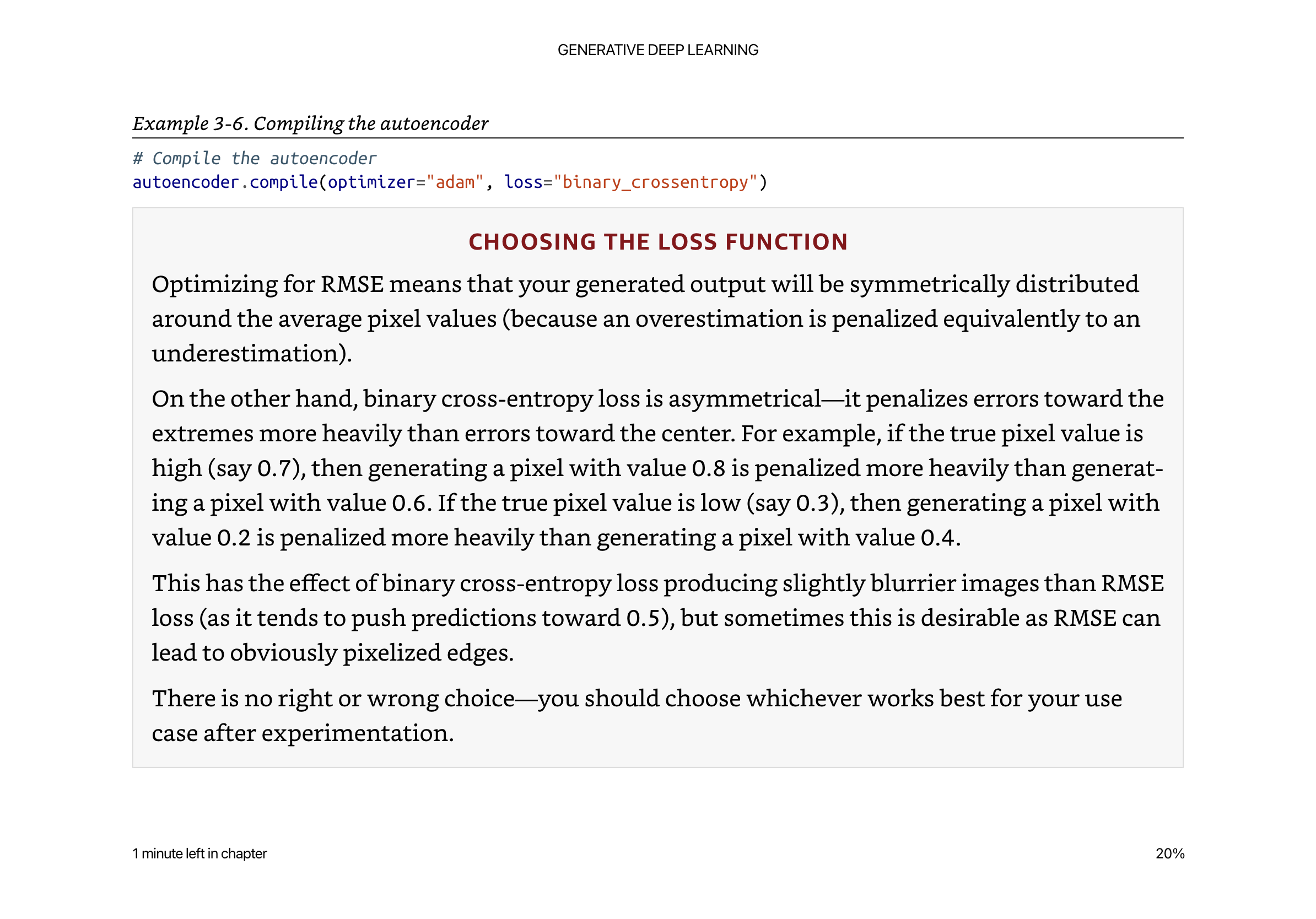
Binary Cross Entropy, a scary looking math equation but let’s break it down.

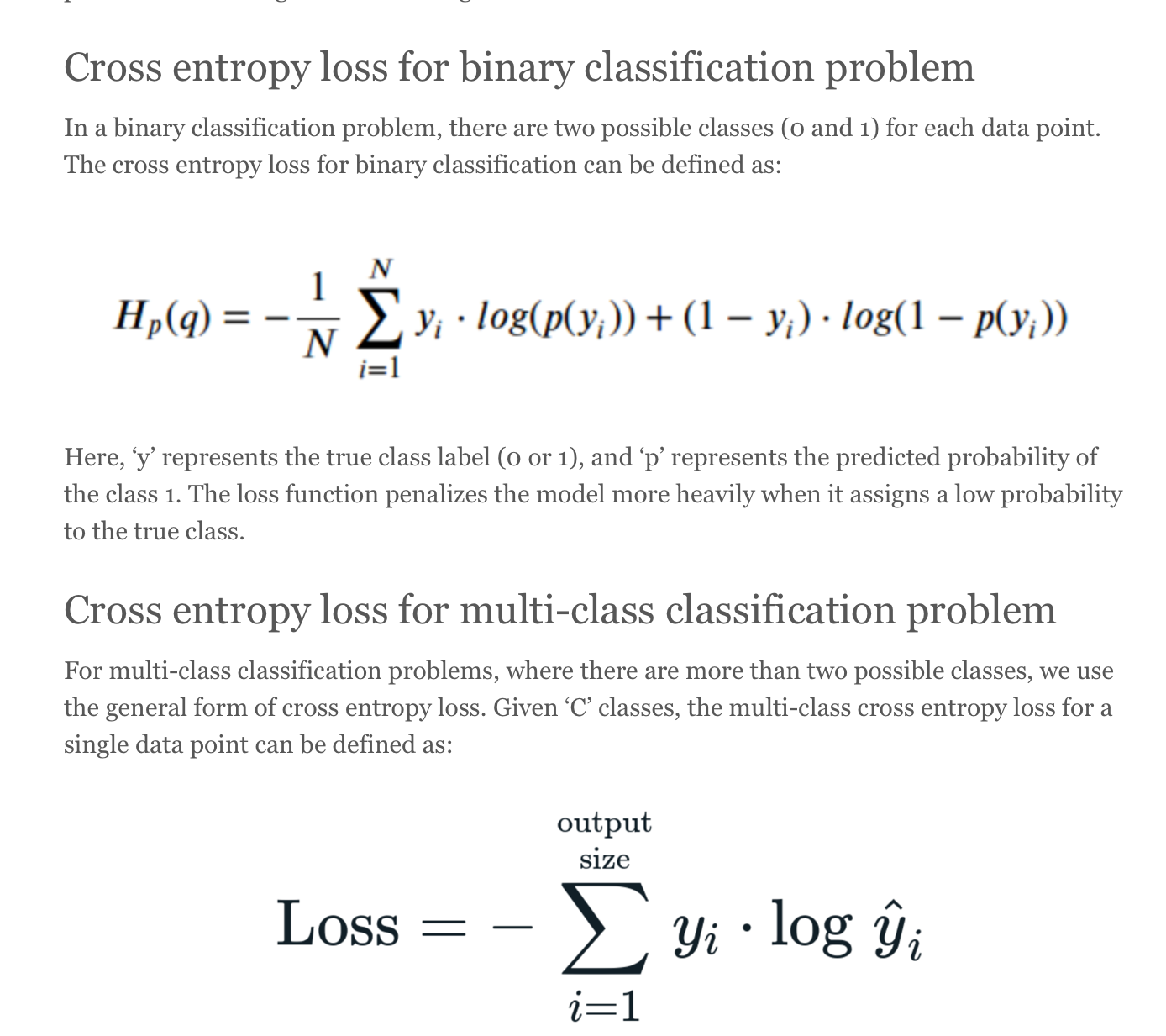
Let yi be our label, p(yi) be our prediction. So if the label is 1 and the prediction is 0.8, we get

1 * log(0.8) + (1-1) * log(1-0.8)
1 * log(0.8) * 0 = -0.09

So really it is saying if we are labeled 1 do log(p(yi)) if we are labeled 0 do log(1-p(yi)).

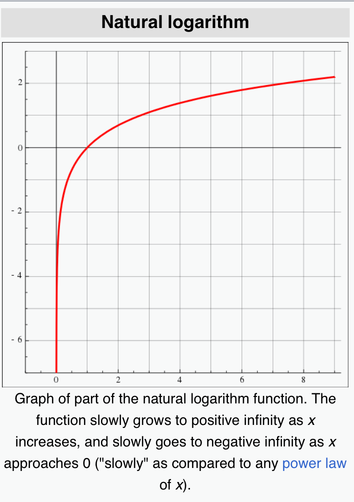
Log just means as x gets get closer to 1, y gets closer to 0. So the closer our loss is to zero, the better we are doing.

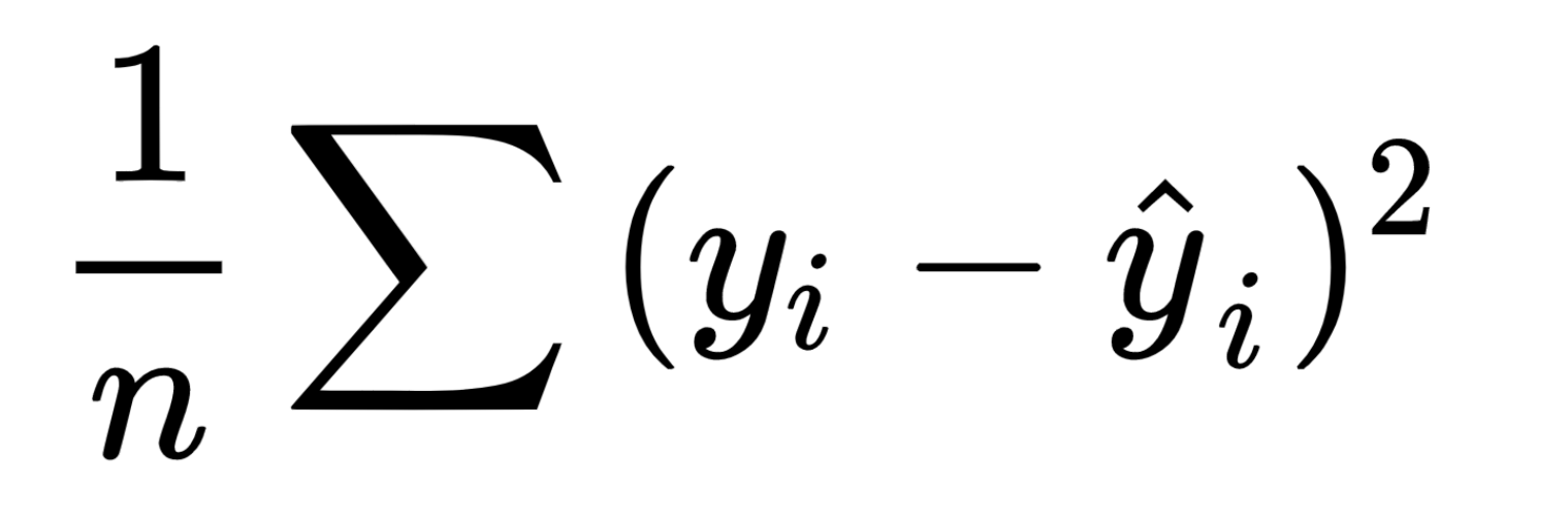
Mean Square Error is a little less intimidating looking of an equation, it’s just taking the difference and squaring it so it is always positive.

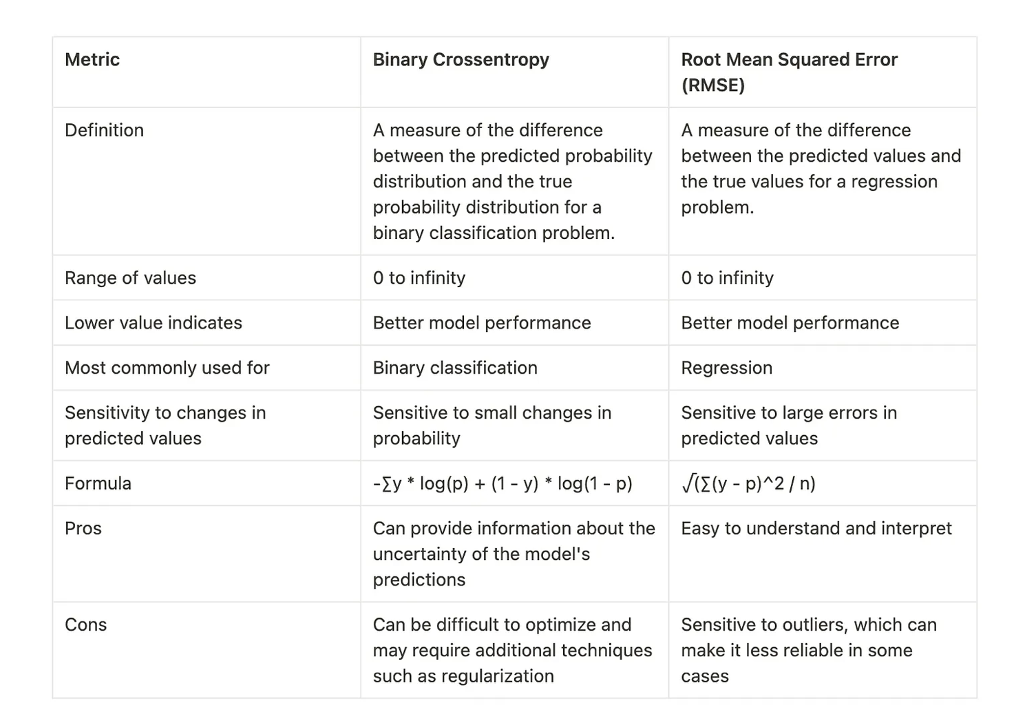
More depth on binary cross entropy vs mean squared error.

When training the auto encoder, below latent space we learn. Each color is a label from Fashion MNIST.

0: Tshirt/top
1: Trouser
2: Pullover
3: dress
4: coat
5: sandal
6: shirt
7: sneaker
8: bag
9: ankle boot

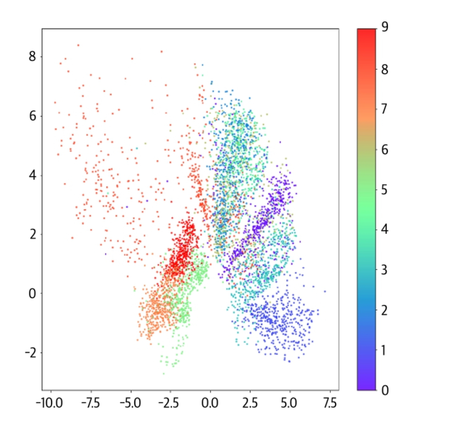
To generate an image, we randomly sample a point from here, and it should generate an image that has those properties.

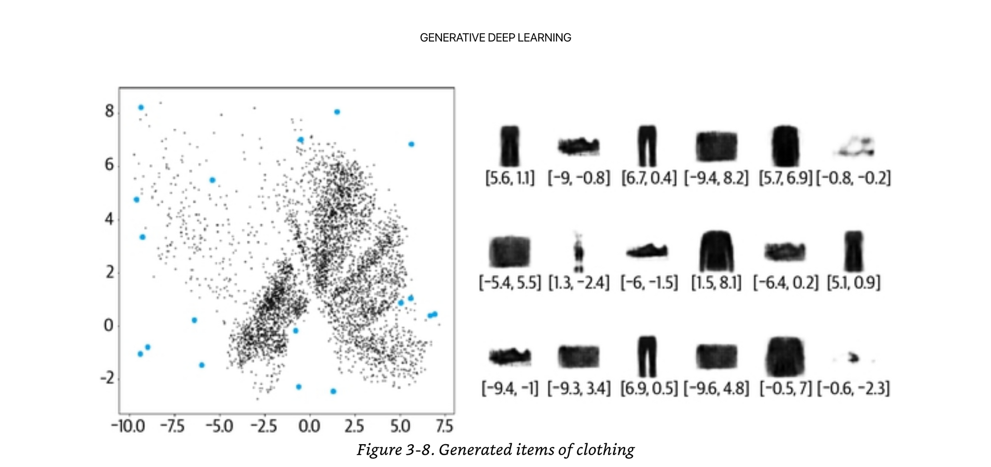
Random sampled points is actually quite hard, because there may not be examples in the space you selected. It is asymmetrical and clustered in various areas.

In order to solve these problems, he introduces the “variational auto encoder”.

Variational Auto Encoder

If you understand what an auto encoder is at the base level, this is a pretty solid fundamental. You can also think of an auto encoder a compression algorithm. The smaller the latent space, the more lossy, which could be a good thing or a bad thing depending on your end objective. Are you trying to get creative? Are you trying to be less lossy? Different objectives could mean different architectures.

The main motivation for the variational auto encoder is restricting where in the latent space points can lie.

Instead of allowing the encoder to place the points anywhere, we have a mathematical constraint that we try to place everything as close to the center as possible, we try to put similar things in a similar area, and the deviation from the center should be as close to 1 unit as possible.

So the encoder instead of picking anywhere, has to run through this function to have things be more likely in the “center”.

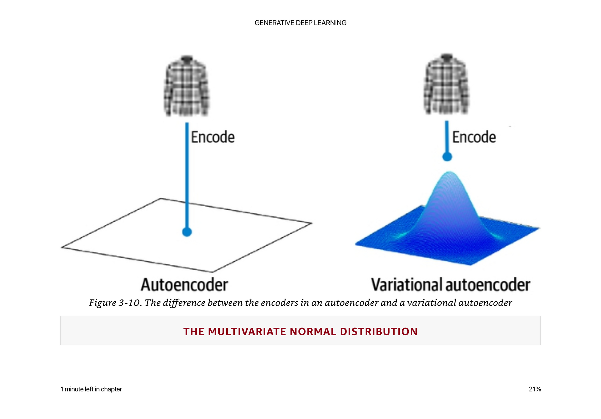
If it was the fashion closet example, everything should be in the middle of the closet, and nothing should be too much farther than 1 meter from the center. If it is, the designer makes you pay extra you because they have to do extra work.

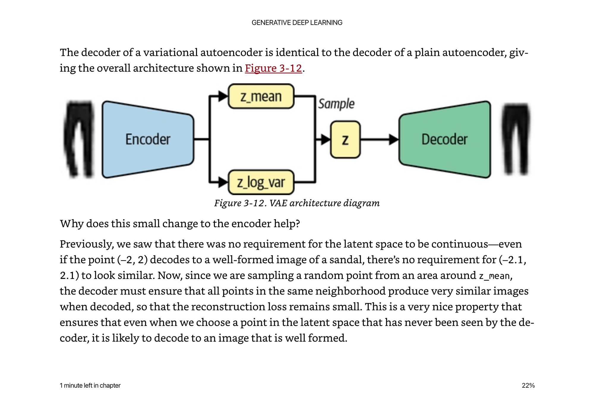
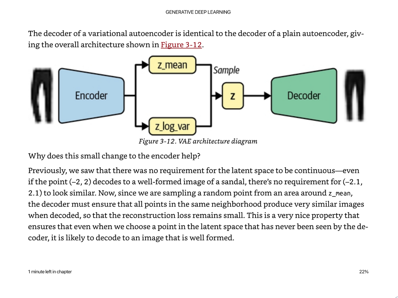
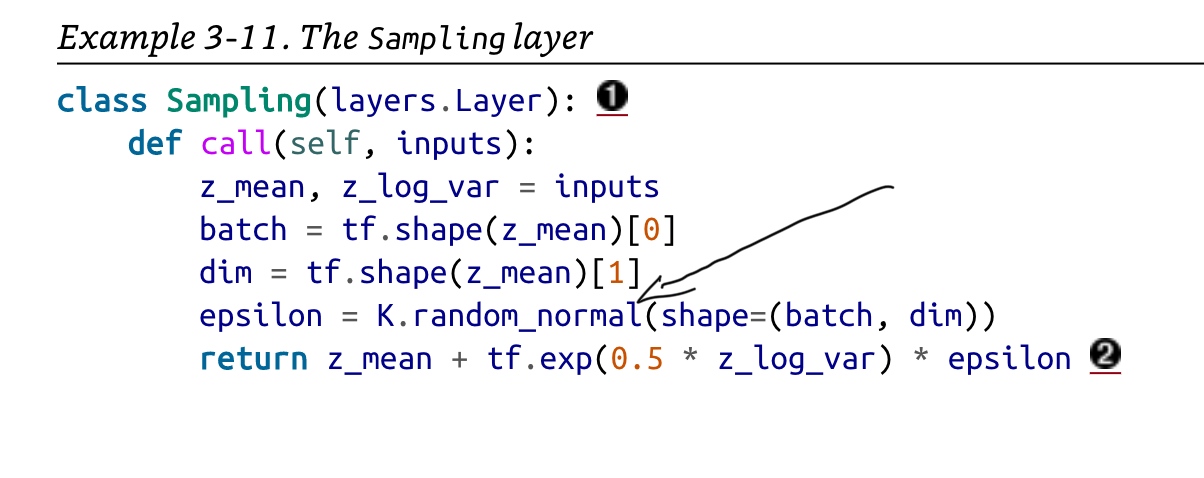
At the end of the encoder, we add this extra “sampling” layer than ensures the latent space can be sampled from a random normal distribution, based on the z_mean and z_variance.

We also have to modify the loss function to add a KL divergence term. Instead of simply looking at the generated pixel values, we look at how well the latent space is organized.

KL divergence is a way of measuring how much one probability distribution differs from another.

We use the KL divergence to penalize the network for encoding observations into a space that differs significantly from that of a standard normal distribution.

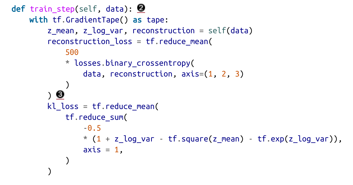
You can simply add the losses together to get a total loss metric.

Kind of funny I drew the mnist example before reading on, and he links to a keras example that does exactly this.

https://keras.io/examples/generative/vae/

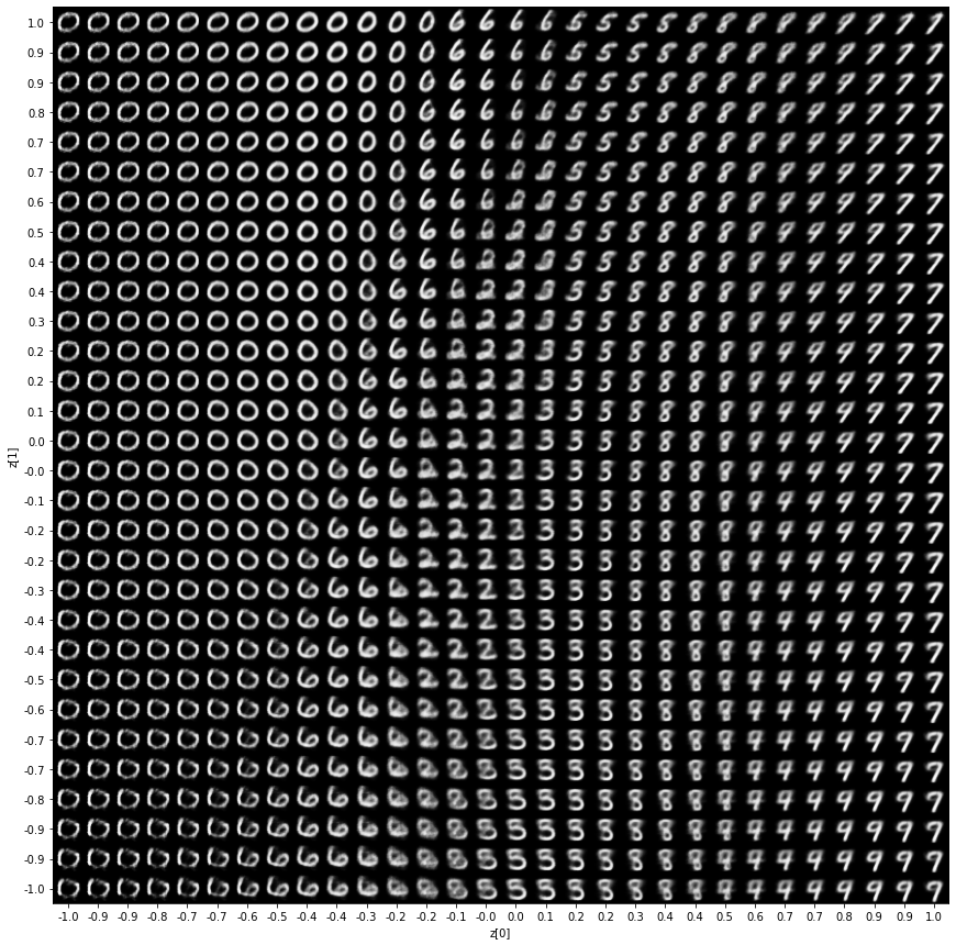
There’s a nice example from mnist where we can see how this constraint organizes the images well.

Retraining the fashion example, now all of our points are closer to the center and more normally distributed. Note how it is not forcing every point to be normally distributed, it is simply penalizing the network if it generates points that are not.

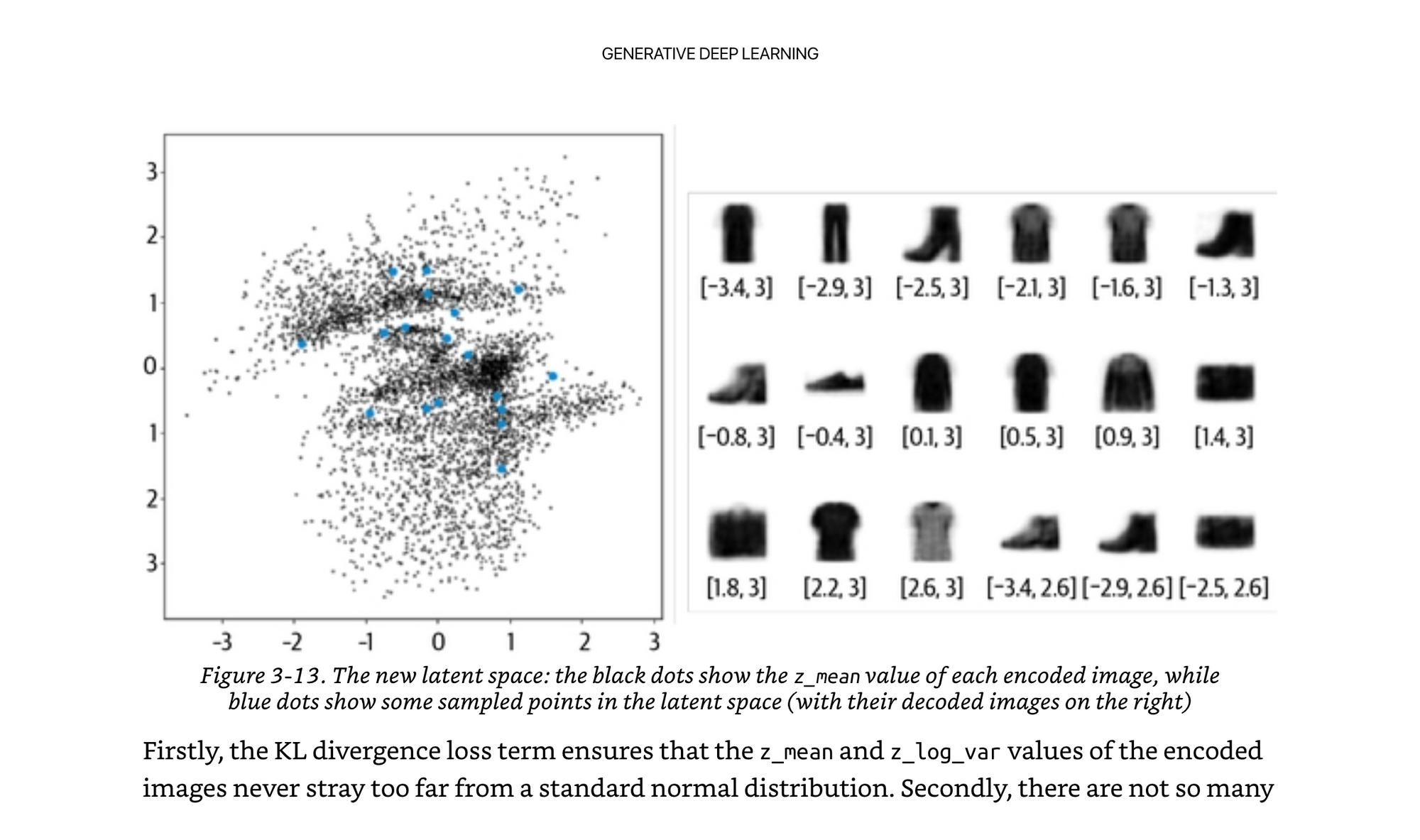
A really cool part to note here…we did not explicitly give the model any labels of “this is a shirt, this is a shoe”, we just enforced it to learn things that were similar and cluster them to similar regions if we want the decoder to work well.

You can take the encoder, and build more supervised learning algorithms on top of it, with less labeled data, because we already learned really good clustering and features.

Training a VAE

We want to generate celebrity faces based on the CelebA dataset.

They increase the latent space from 2 to 200 so that the network can encode more information of the details of the images.

Just want to point out lines like this… increasing from 2 to 200 and other hyper parameters are chosen.

We increase the factor for the KL divergence to 2,000. This is a parameter that requires tuning; for this dataset and architecture this value was found to generate good results.

It’s like these crazy “rule of thumb” math tricks that make training neural networks hard. If not documented well, it is hard to reproduce, even given the data.

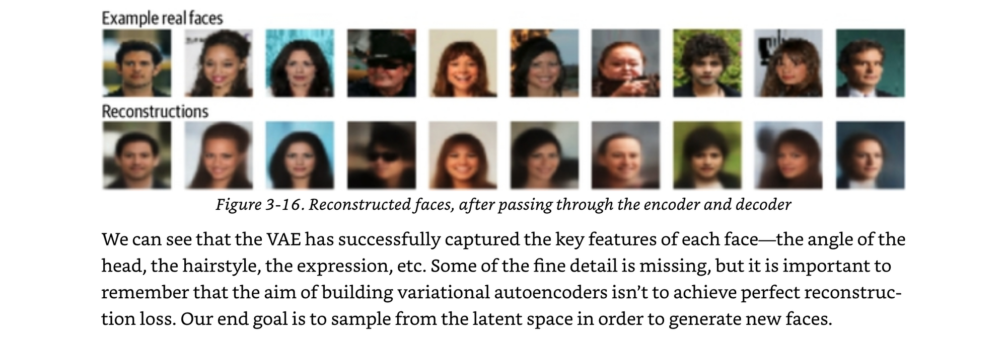
Below, you’ll see that the images are a little blurry, partly due to the loss function we have chosen. Mean squared error between pixel values + KL divergence of the z_mean and z_std variables within the encoder. This means we can sample from the space well, and the pixel values will be roughly in the correct place, which is actually pretty good for cropped faces where there actually isn’t too much variation in what you have to generate. The nose is in the middle, sometimes it’s facing left, sometimes right, sometimes add hair, sometimes change the background color etc.

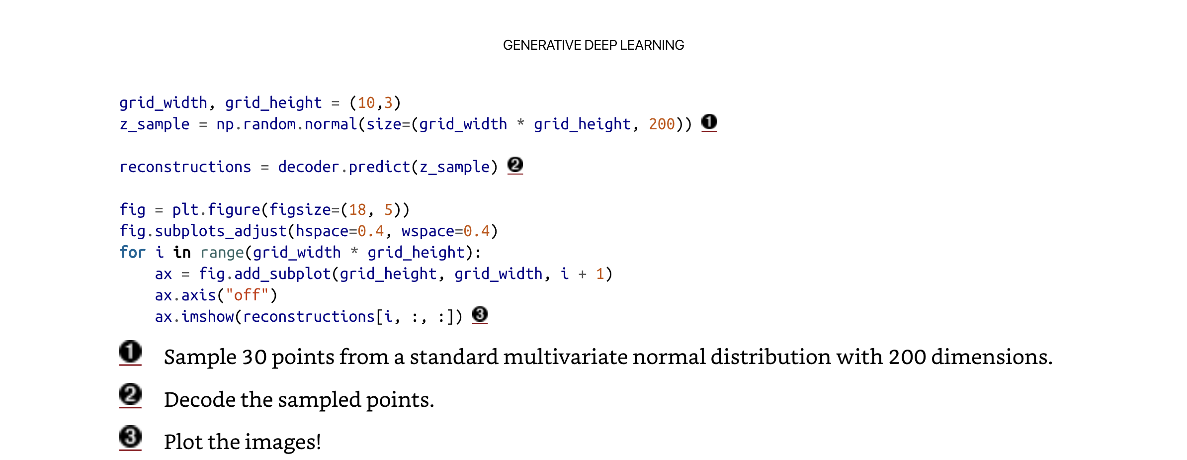
Sampling

Our end goal is to sample from the latent space in order to generate new faces.

For this to be possible, we should be able to look at the variables in the latent space and see that they look like standard normal distributions.

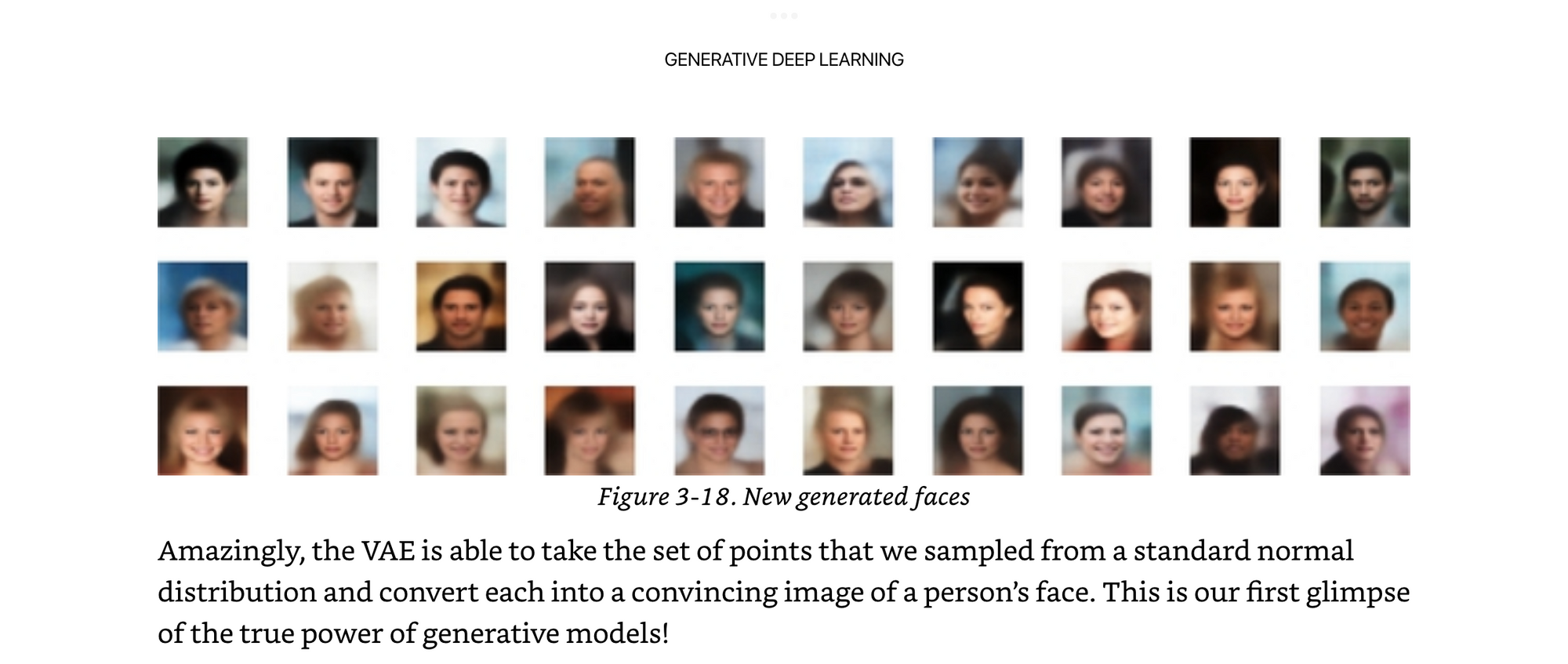
With a little bit of code, we get out some blurry faces!

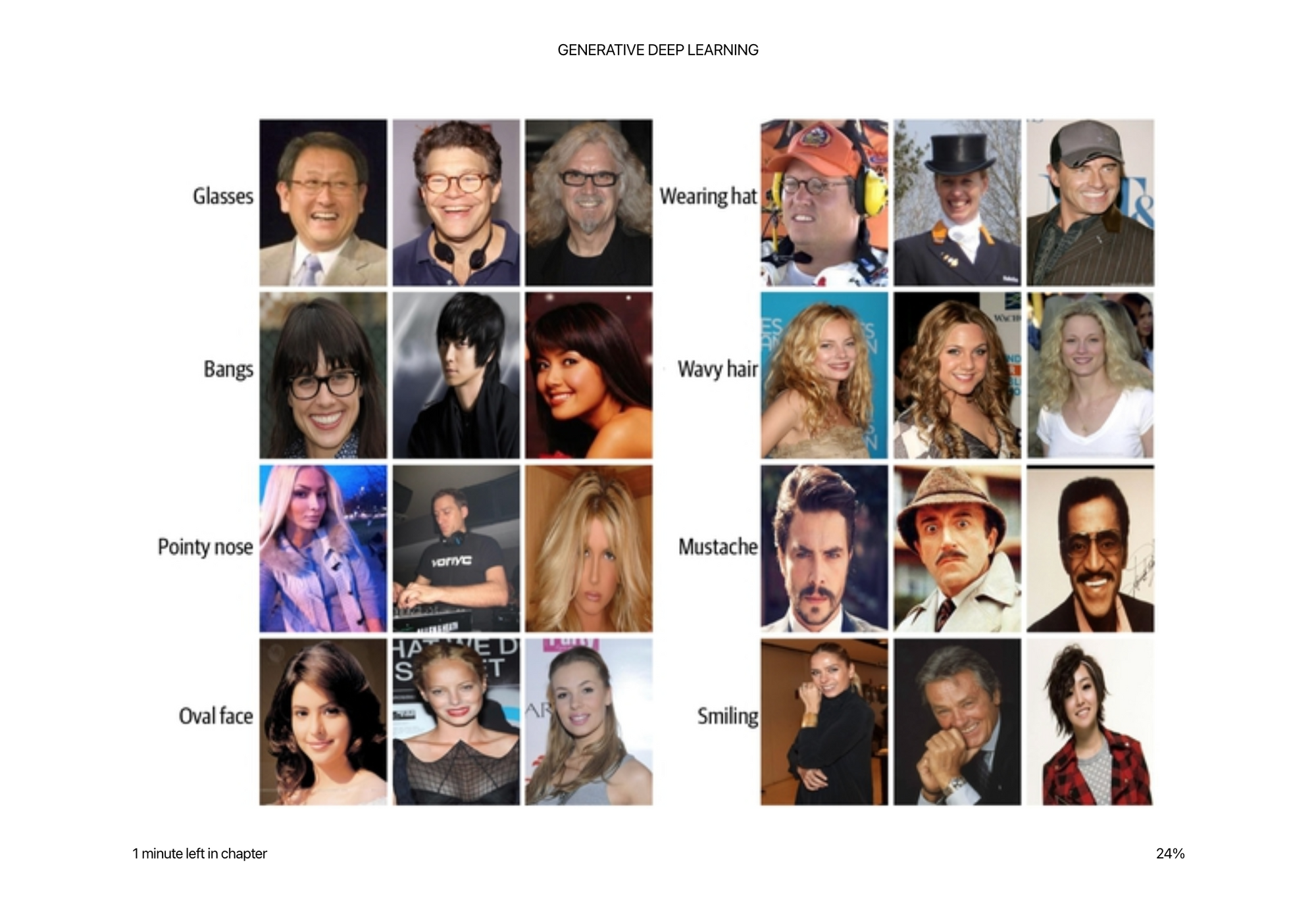
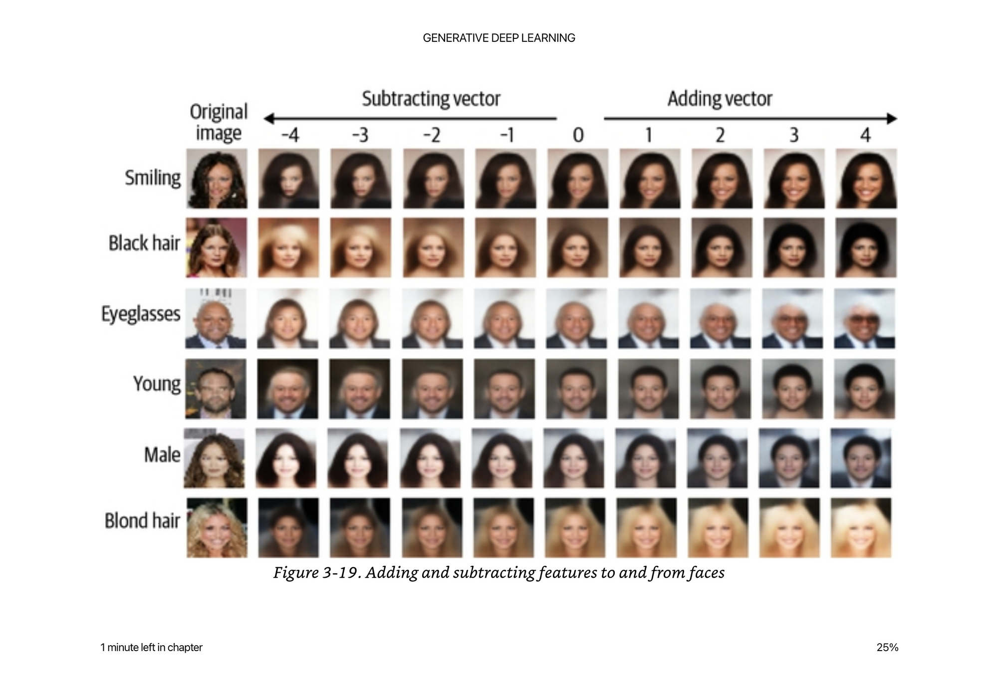
Latent Space Arithmetic

If we can find an example of a latent space vector where someone is smiling, and add it to the latent space vector of an image where someone is not smiling, we can generate a “more smiley” version of the original image.

Z_new = alpha * z_smile + z_orig

You can also do the same thing morphing between faces:

z_new = z_A * (1- alpha) + z_B * alpha

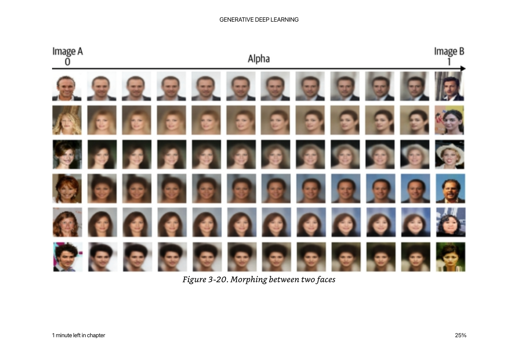
The smoothness of the transition is a key feature of a VAE because we are enforcing that the latent space is continuous normal distribution, even if there are many features (eye color, hair color, etc)