Generative Deep Learning Book - Chapter 4 - Generative Adversarial Networks (GANs)

Greg Schoeninger

Jun 15, 2023

Join the Oxen.ai "Nerd Herd"

Every Friday at Oxen.ai we host a public paper club called "Arxiv Dives" to make us smarter Oxen 🐂 🧠. These are the notes from the group session for reference. If you would like to join us live, sign up here.

The first book we are going through is Generative Deep Learning: Teaching Machines To Paint, Write, Compose, and Play.

Unfortunately, we didn't record this session, but still wanted to document it. If some of the sentences or thoughts below feel incomplete, that is because they were covered in more depth in a live walk through, and this is meant to be more of a reference for later. Please purchase the full book, or join live to get the full details.

Generative Adversarial Networks

In the book he talks about "Brickki" - the bricks company. This company creates bricks on an assembly line. A competitor has launched a product copying their bricks. They start to add people to check bricks (discriminators) that come through to make sure they are not forged bricks. The forger (generators) updates their process so they are even more indistinguishable. And onward and onward until you can’t tell real from fake.

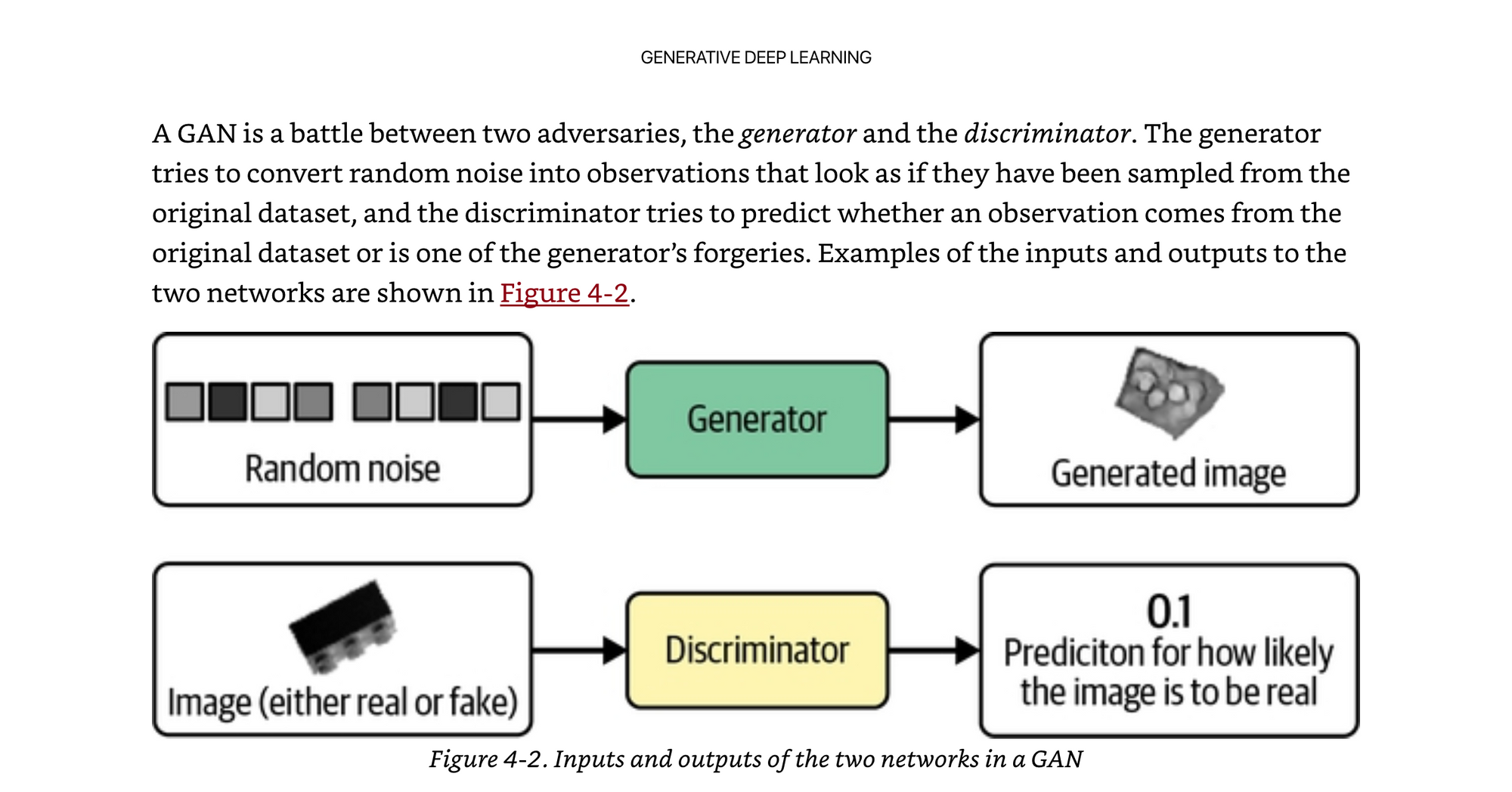
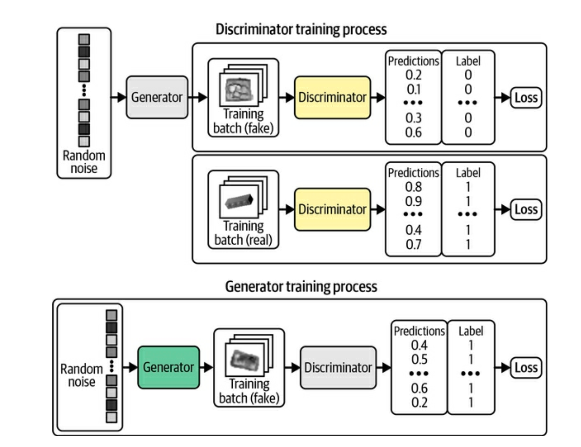
The basic idea behind a GAN is you have one neural network that is taking random noise, and generating an image, and another neural network that is looking at a mixture of real images, and generated images, and trying to distinguish the difference. The first network is called a Generator, and the latter a Discriminator. They are jointly optimized so that as one improves at generating, the other improves at discriminating. They battle back and forth until they reach an optimima.

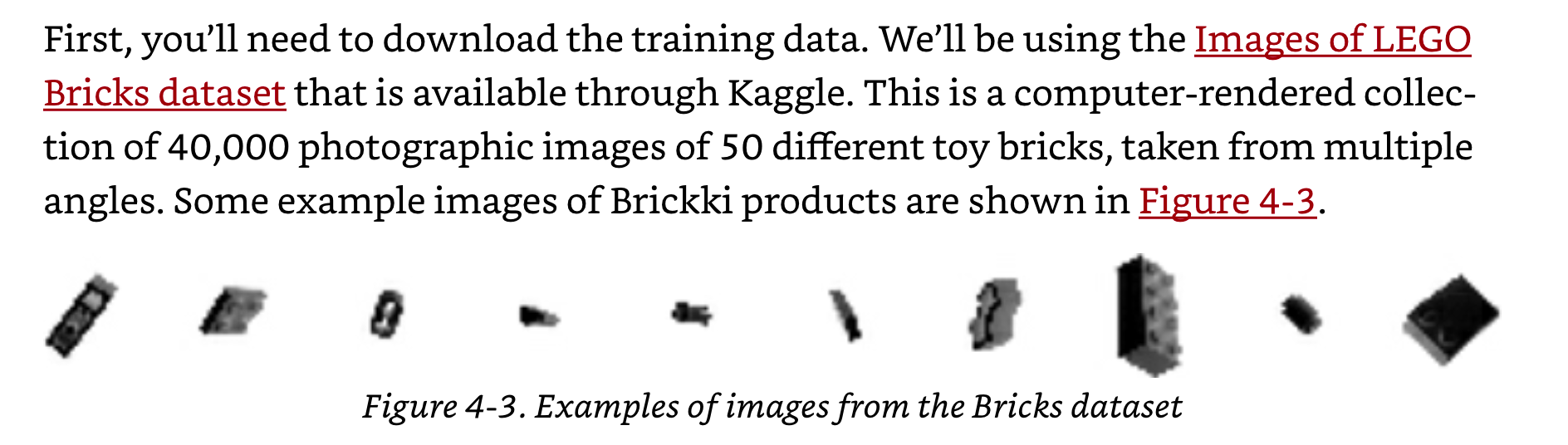
They use a LEGO bricks dataset - 40,000 computer generated images of bricks from different angles as the training data. Which is kind of funny, because if you think of it…they have a 3D model of a brick, they created this dataset from, and rendered it with a 3D graphics engine, and now we are trying to replace that graphics engine with a neural network…but we can already generate the perfect image from the graphics engine. So kind of a toy example.

The graphics engine already had all of it’s parameters of x,y,length,height,camera angle, etc…that is a pretty freakin compact representation, but the graphics engine is not flexible about what it can generate from that representation. But enough complaining about the example data.

The full code in Keras for a Deep Convolutional GAN (DCGAN) can be found here:

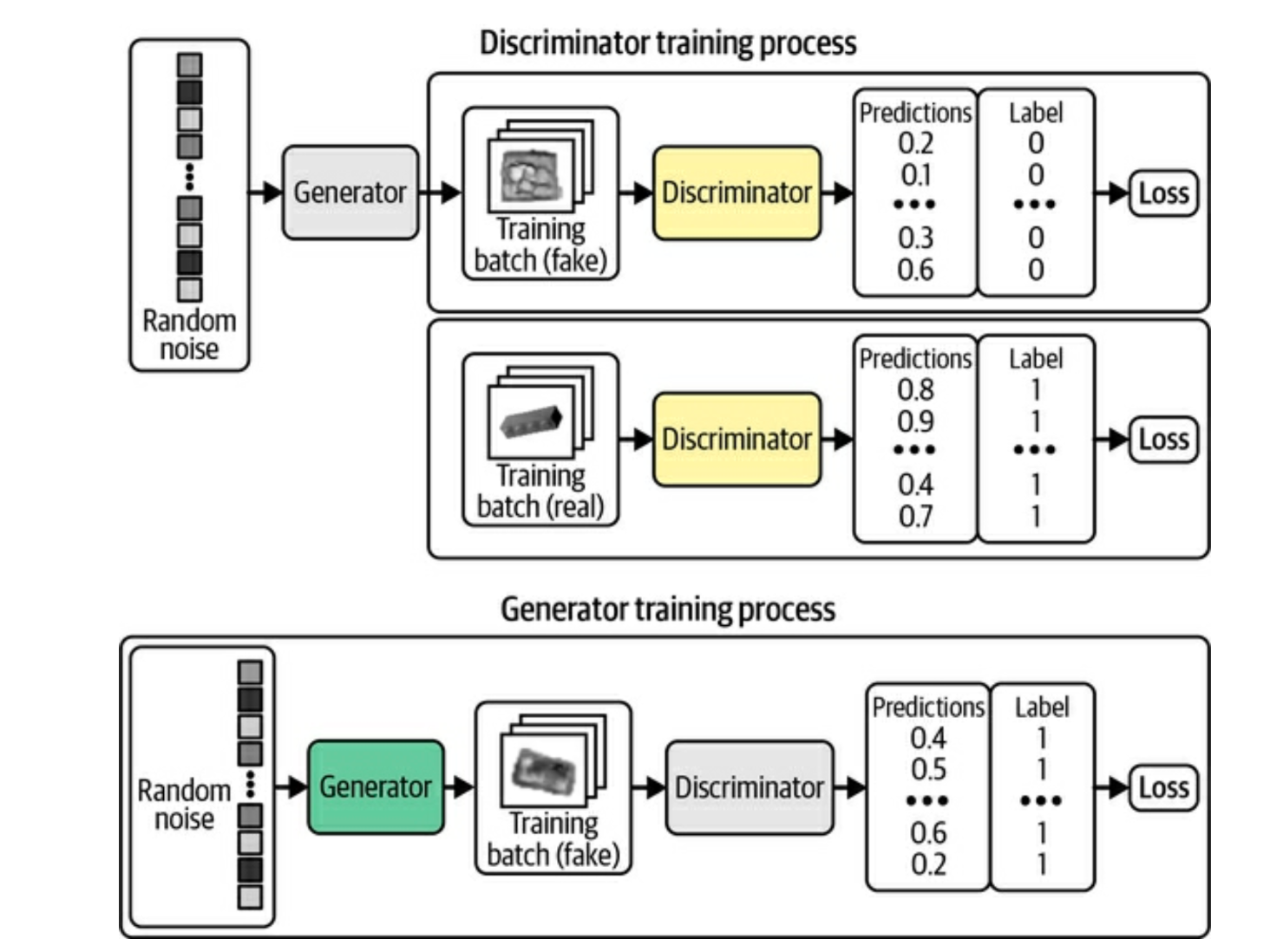
Below is a deeper look at what the inputs, outputs, and labels look like for the discriminator and the generator.

You can see as the training progresses, the images go from blobs to more and more looking like bricks.

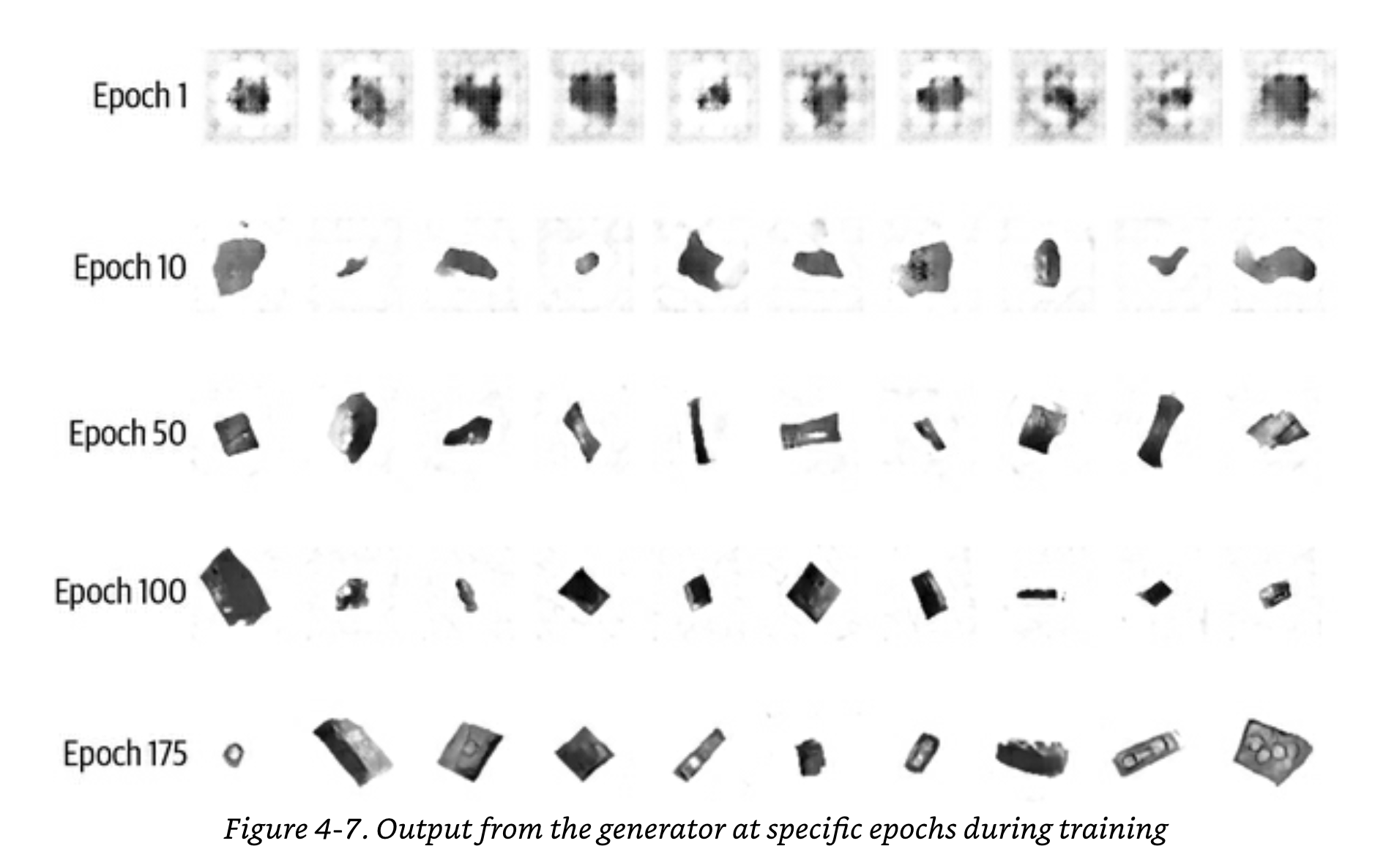
“It is somewhat miraculous that a neural network is able to convert random noise into something meaningful. It is worth remembering that we haven’t provided the model with any additional features beyond the raw pixels, so it has to work out high-level concepts such as how to draw shadows, cuboids, and circles entirely by itself”

GANs can be tricky to optimize

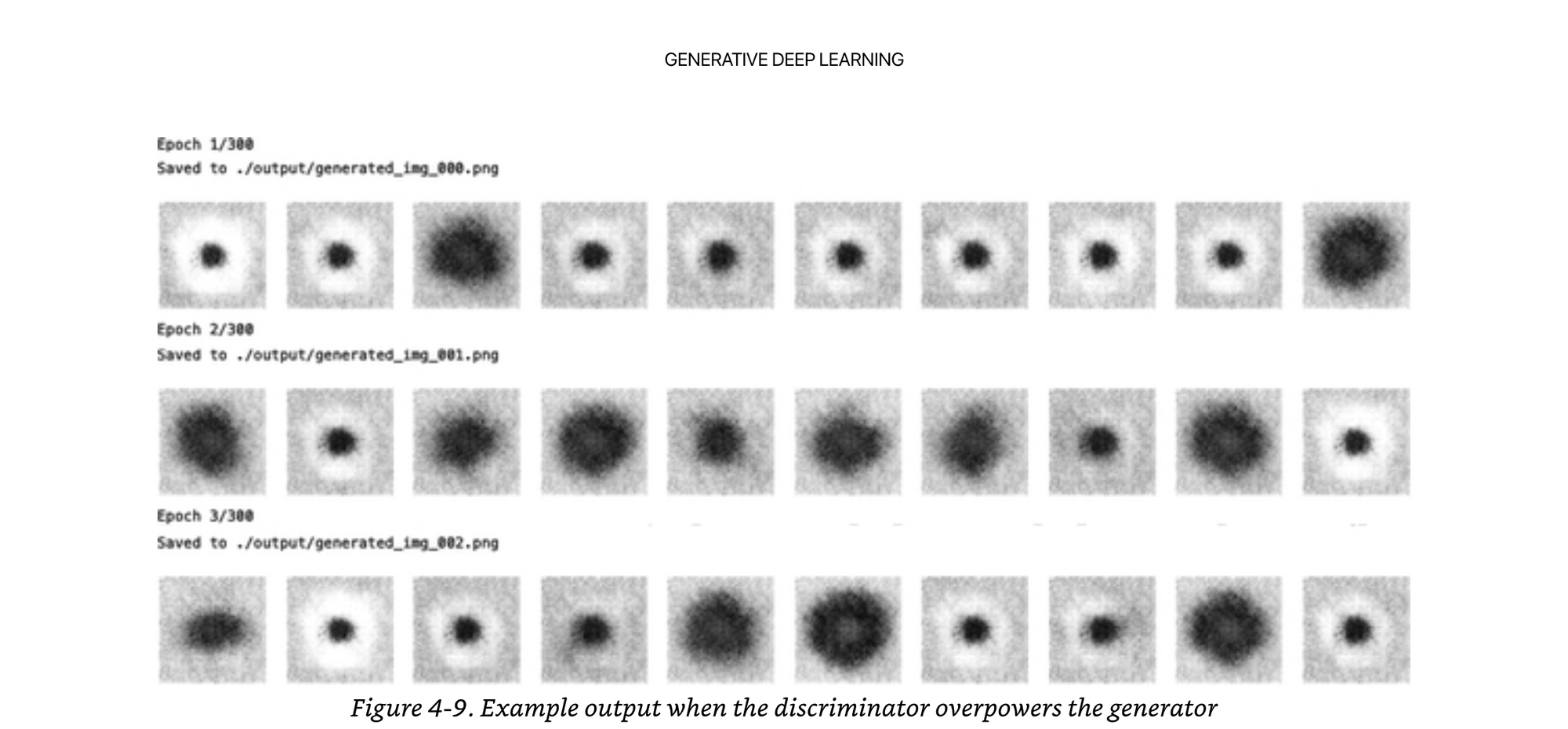
There is a balance of training and optimizing the discriminator to not overpower the generator, because if it always is correct, then the generator can never learn what will trick it. One way to help do this is add some random noise to the labels of the discriminator.

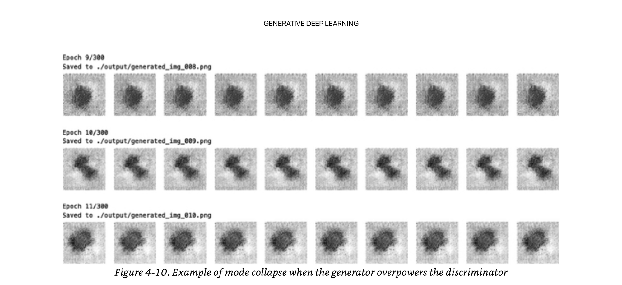
The opposite can be true as well if the generator overpowers the discriminator. This is called “mode collapse”, where the generator knows one specific type of image that always fools the discriminator, and never generates anything else besides this one trick that the discriminator never learns.

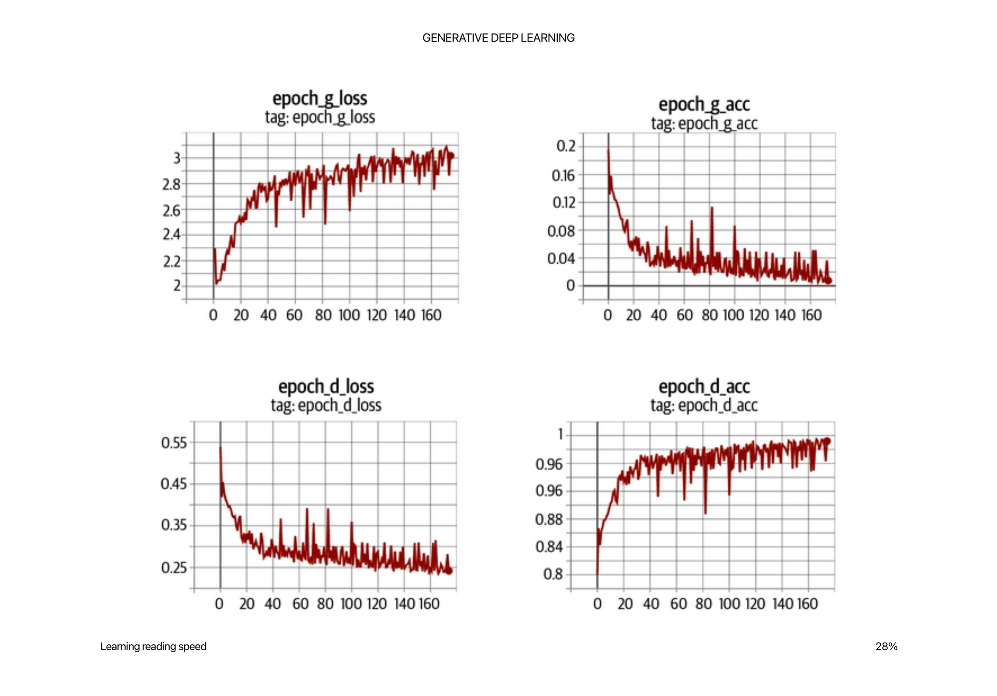
GANs can be hard to evaluate merely by loss function

Since the generator is only graded against the current discriminator and the discriminator is constantly improving, we cannot compare the loss function evaluated at different points in the training process. Indeed, in Figure 4-6, the loss function of the generator actually increases over time, even though the quality of the images is clearly improving. This lack of correlation between the generator loss and image quality sometimes makes GAN training difficult to monitor.

There are also many hyper parameters to tweak in a GAN and trying to balance all of them is more of a mathematical art then a science right now. You can definitely learn intuition though.

This is another example where a “vibe check” from your models is honestly not the worst metric.

Wasserstein GAN with Gradient Penalty (WGAN-GP)

The two main problems the Wasserstein GAN solves are

defining a meaningful loss metric
Stabilizing the training process so we don’t have mode collapse or “discriminator overload” (do they have a term for this?)

The loss function is the key again.

First it switches the labels from 0,1 to -1,1 so that we can have outputs in the range from -infinity,infinity instead of 0,1.

Since it is no longer 0,1 and it is more of a score, we call it the “critic” instead of the discriminator.

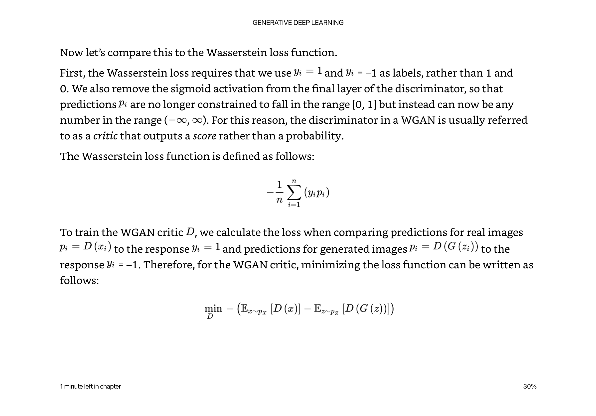
All this is saying is the critic (discriminator) tries to maximize the difference between its predictions for real images and generated images.

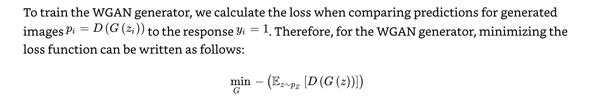
Then the generator tries to produce images that are scored as high as possible by the critic (it wants the critic think they are real).

Since the outputs from the critic can be infinite, we need some way of constraining their values. This is where the Lipschitz Constraint comes in. Neural networks can “explode” when numbers get too big because of floating point math.

Essentially, we require a limit on the rate at which the predictions of the critic can change between two images (i.e., the absolute value of the gradient must be at most 1 everywhere).

Deeper dive here: https://jonathan-hui.medium.com/gan-wasserstein-gan-wgan-gp-6a1a2aa1b490

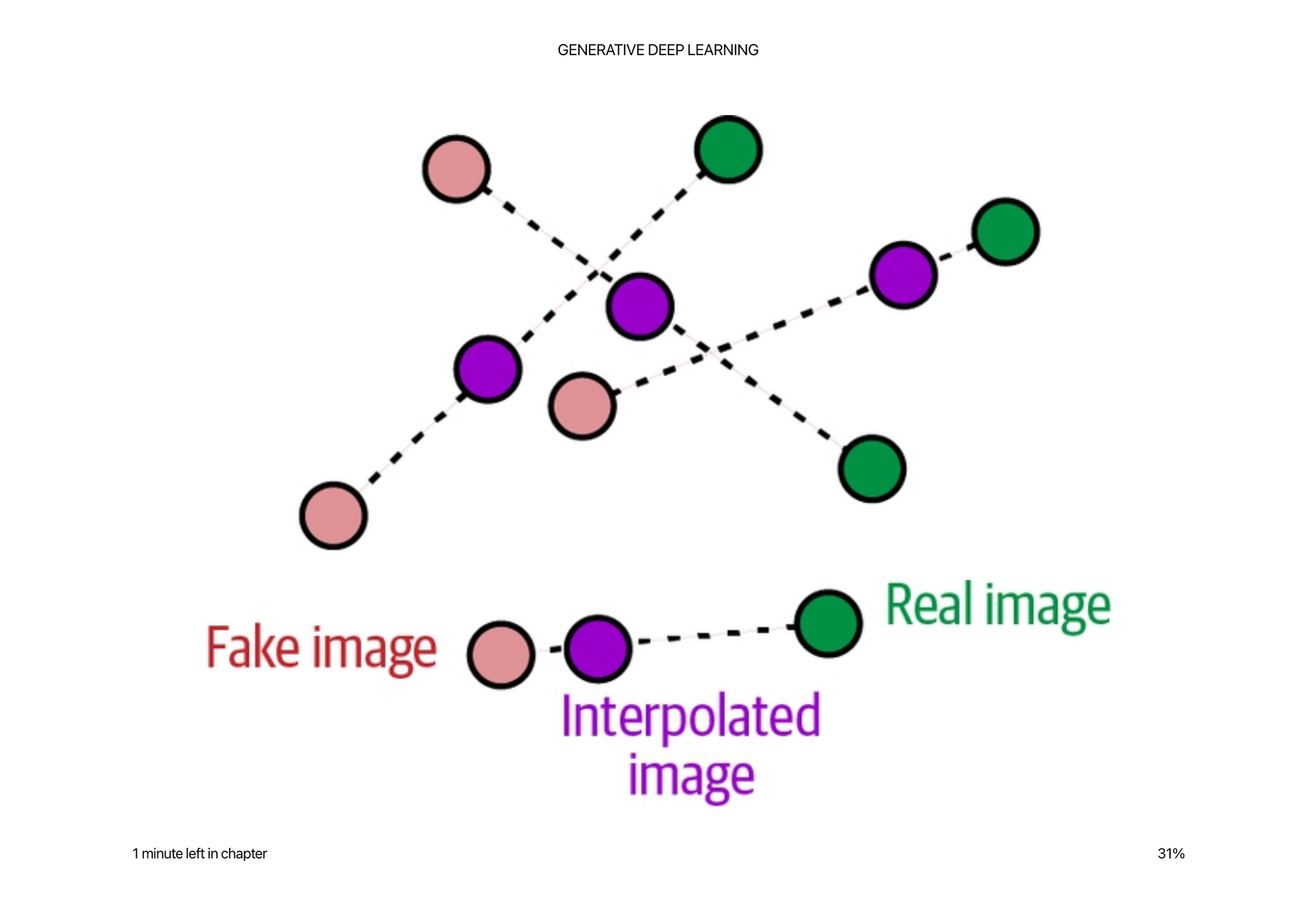
So it is pretty crazy how they approximate this constraint… It is not tractable to calculate this constraint everywhere… So they randomly generate these interpolated images between the real and the fake images, the critic is asked to score these randomly sampled images, and then they make sure that the critic does not update it’s weights too much in any direction given these images.

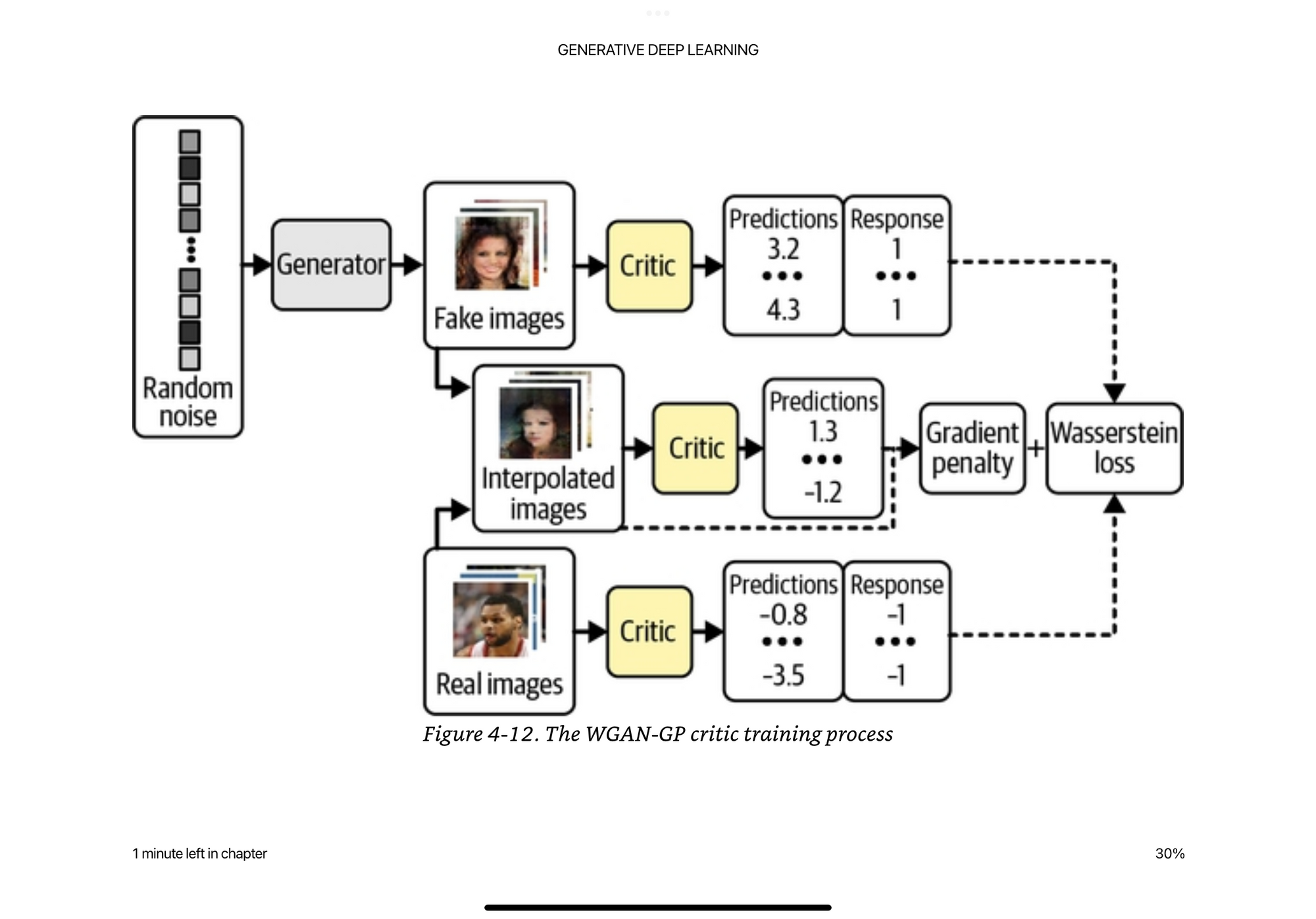
This requires we train the critic several times between each time we train the generator, a typical ratio is 3/5. Which is also some magic number-ness.

Again, another point to drive home, is look at this crazy math that is required to even come up with this loss function to try to improve the model…Let the PHDs come up with this, let everyone else iterate on the data.

GANs typically have sharper edges and more well defined images than VAEs. Even though still not perfect as we can see.

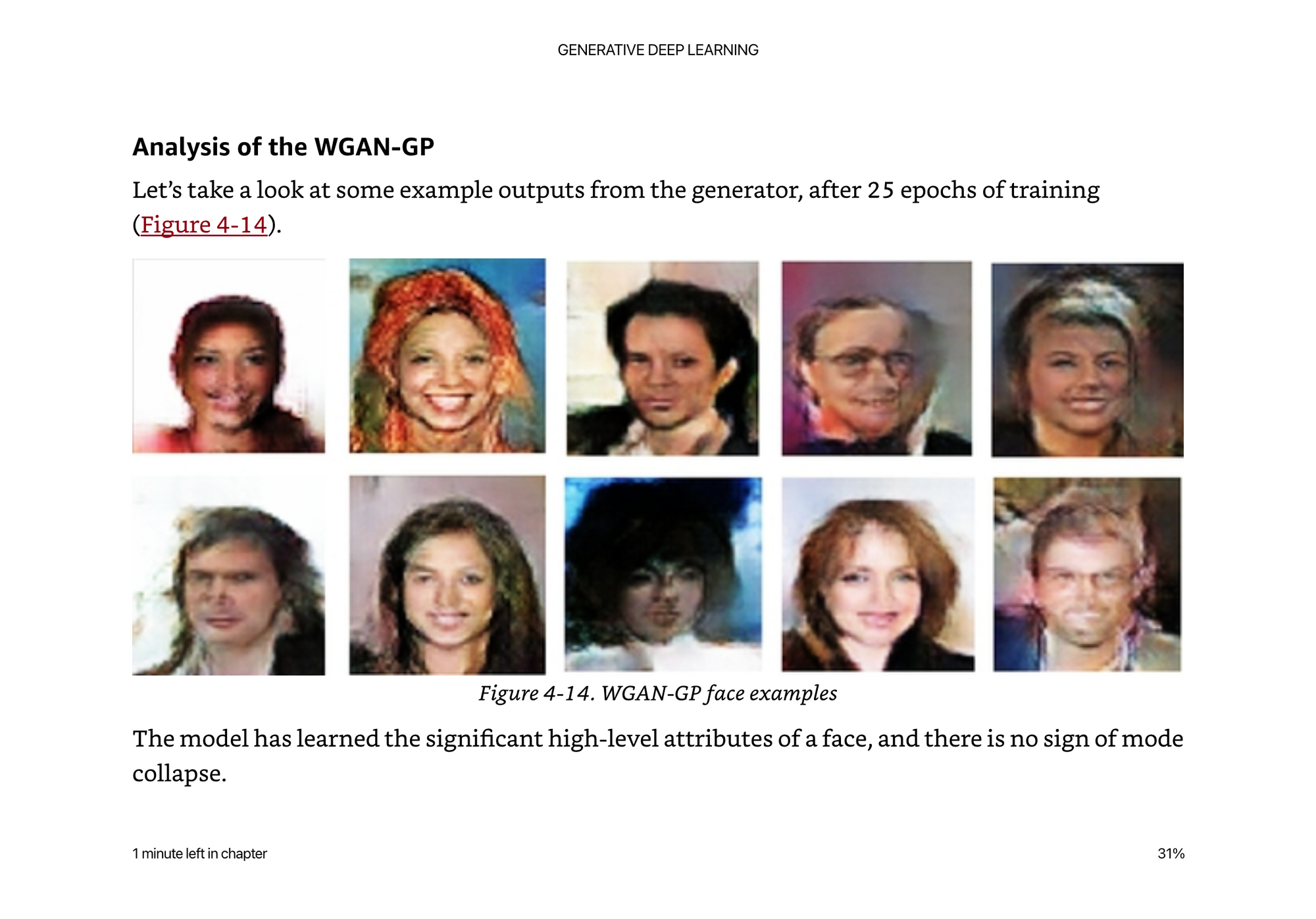
It is also true that GANs are generally more difficult to train than VAEs and take longer to reach a satisfactory quality. However, many state-of-the-art generative models today are GAN-based, as the rewards for training large-scale GANs on GPUs over a longer period of time are significant.

Conditional GAN (CGAN)

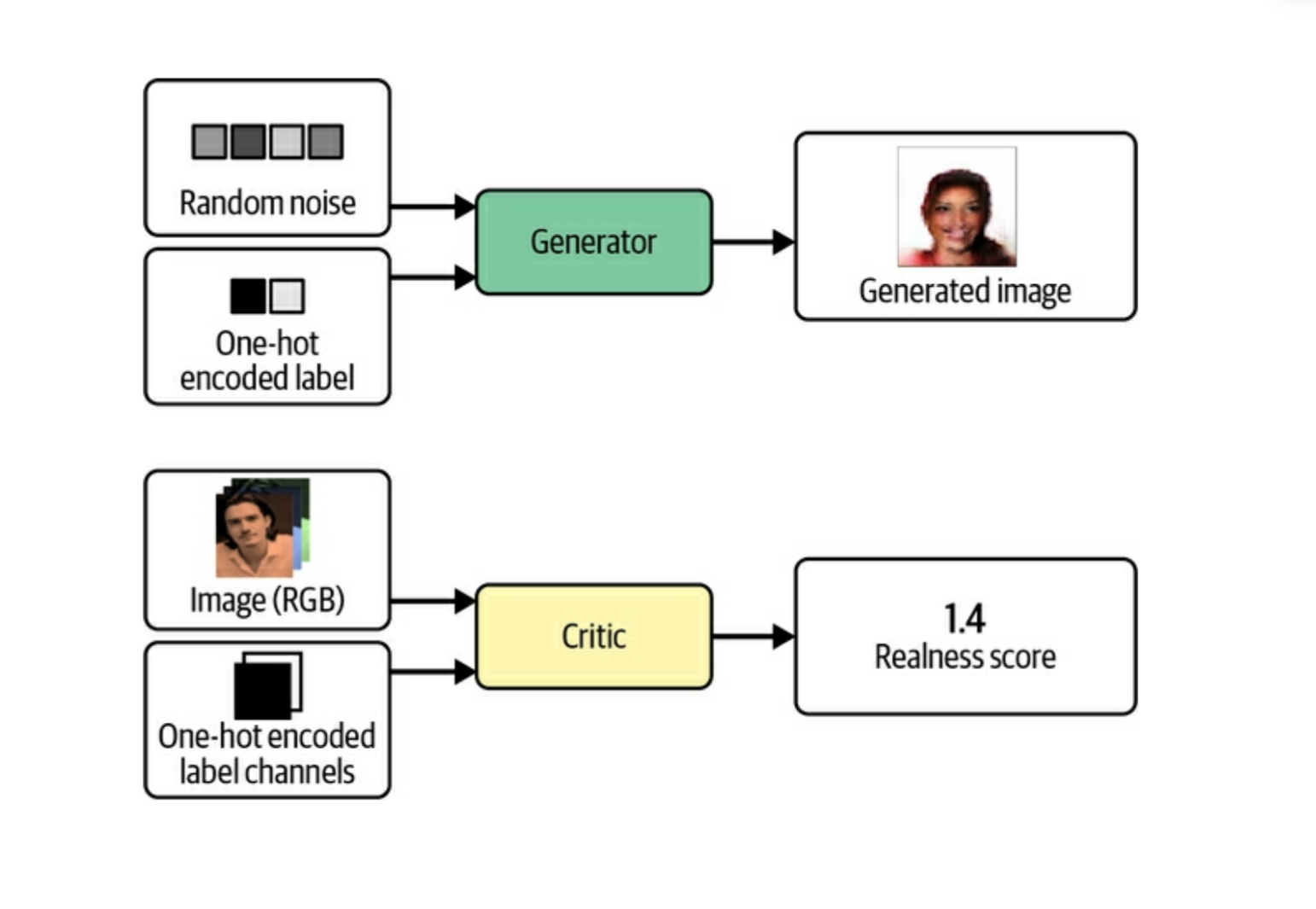
Conditional GANs have a simple tweak that they pass in a one hot encoded vector to along with the random noise vector into the input, as well as using one of the channels of the input image to the critic as information about the label or condition.

In the example in the book, they take the isBlond feature from the training data and make a binary encoded one hot vector as input. They could have also done this with all the features from the CelebA dataset to make a longer vector with more features that you would want to apply to the output.

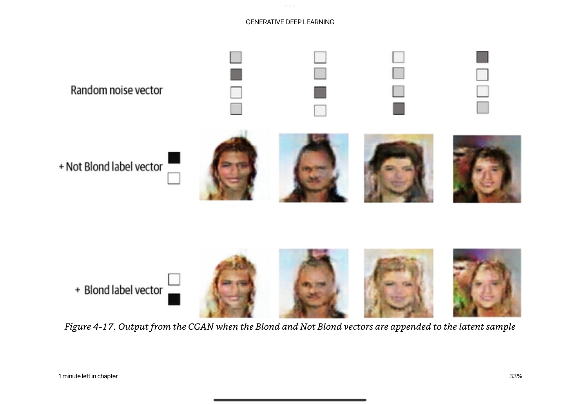
You can see the generated images above, given the same random noise vector, generate structurally a very similar image, just changing the colors around the hair.

Obviously we are still far away from the diffusion models we see today, but it’s cool to see how you can control the latent space with some smart data processing and injection into the model and training process.