Join the Oxen.ai "Nerd Herd"

Every Friday at Oxen.ai we host a public paper club called "Arxiv Dives" to make us smarter Oxen 🐂 🧠. These are the notes from the group session for reference. If you would like to join us live, sign up here.

The first book we are going through is Generative Deep Learning: Teaching Machines To Paint, Write, Compose, and Play.

Unfortunately, we didn't record this session, but still wanted to document it. If some of the sentences or thoughts below feel incomplete, that is because they were covered in more depth in a live walk through, and this is meant to be more of a reference for later. Please purchase the full book, or join live to get the full details.

Autoregressive Models (LLMs and More)

Auto regressive models are well suited for generating sequences of data, which naturally fits text, but can also be applied to images if you think of the pixels as a sequence as well.

Autoregressive models condition predictions on the previous examples in the sequence, rather than on a latent random variable. They try to explicitly model the data generating distribution.

Ge uses the example of a prison in which the prison warden wants to write a novel. He then gets all of his prisoners in a cell, and tells them the previous word in the novel, and that he wants them to generate the next word. Each prisoner has their own ideas, thoughts, and opinions that they can feed to the guard at the door, who will eventually tell the warden the collective decision for the next word. The warden tells the guard if the next word is correct, who relays the information to the prisoners, who can update what they know they story is about, and get back to generating the next word. Eventually this process gets better and better at knowing what the story is about, and predicting the next word.

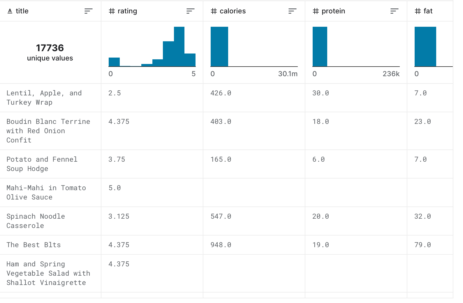
Epicurious Recipes Dataset

Working with Text Data

Text is made of discrete chunks or values of characters or words. Unlike pixels where there is a smooth transition between the underlying red, green and blue values, with discrete characters or words there is no smooth transition to get you from “cat” to “dog”.

Text data has a time dimension, whereas images have two spatial dimensions. Video kind of combines the two. But text does not have the spatial invariance that images have, you can’t flip a sentence around and have it mean the same thing, where you can do this with an image.

With language there are long term dependencies and you might need to know the first word to predict the last, or in machine translation sometimes you need to know the last word to predict the correct version of the first (this is why real time speech translation is hard, because you have to listen to the context to fully understand, luckily we as humans already have a ~200ms delay in our reaction time to inputs so it can feel like real time to us)

Text data is highly sensitive to changing the individual units, unlike images where shifting a pixel slightly will not change the overall meaning, text changing one character could make the entire sentence gibberish. Every word and character is vital to the meaning of the sentence.

Text data does have some inherent grammatical and syntactical rules that can be followed, but also have semantics that do not rely on the syntax, that can be harder to model. For example “The cat sat on the mat” follows good syntactical structure, and so does “I am in the beach”, but the latter does not have proper semantics because a “beach” is not something you can be “in”, even though it is grammatically correct to put a noun there.

The couple I will add that I always think are interesting

The same sentence, the same physical words, said at a different pace or with emphasis on different words can mean something completely different. The first implies someone else stole the jewelry, and the second implies that he stole something else.

HE didn’t steal the jewelry

He didn’t steal the JEWELRY.

The same sentence or word can mean different things in different contexts. Not just context of the surrounding sentences, but the context of the person reading it, and their entire life history. Some sentences, books, quotes, really resonate with certain people because they see some deep meaning in it that others do not and vice versa. Language is an imperfect compression technique and way to communicate ideas.

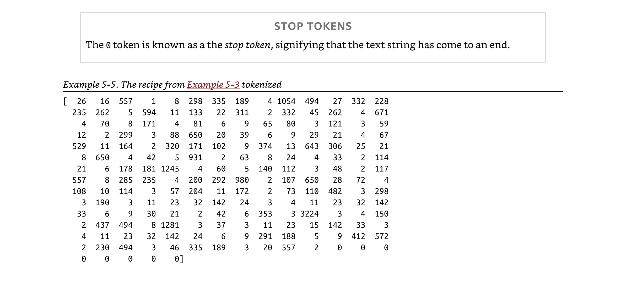
Tokenization

Tokenization is the process of splitting the text up into individual units, such as words or characters or subwords.

There are many considerations to take into account when tokenizing.

• Capitalization or not, sometimes there is value in knowing a letter is capital, sometimes it just adds too much complexity for the model to learn given the size of the data.
• If you do tokenization at the word level, it is likely that you will have words that are seen only a few times in the training data, it is often better to just replace these with “unknown” and say “John UNK went to the market” and let the model infer that it is a last name, rather than try to learn every single last name of every person.
• Knowing what punctuation is important to keep where can be hard. Ex) Dr. Sue lives in the U.S.A. And who’s favorite book is Lord of the Rings, The Twin Towers
• If you use words it will never be able to generate a word it’s never seen.
• You can use subwords like prefixes and suffixes and lemmas.
• Learning at the character level requires less options to output, hence less weights, but can be much harder to learn meaningful abstractions rather than syntactical patterns.

Tokenized text looks just a like a list of indices that you will use to look up into a table of embeddings for input, and can be used as a N way classification problem on output.

If you have 10,000 word vocabulary (which is rather small and leaves out a lot of words) and a 100 length embedding to represent each word, that is already 1,000,000 parameters to learn.

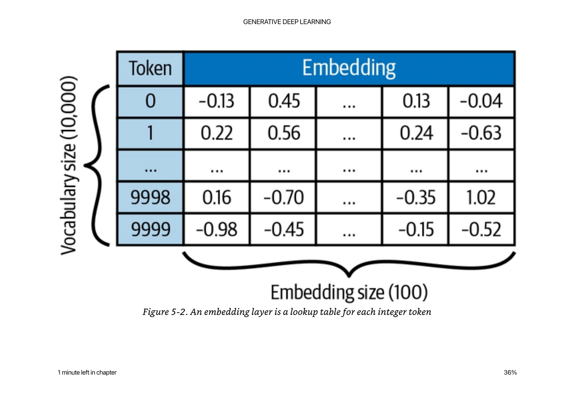
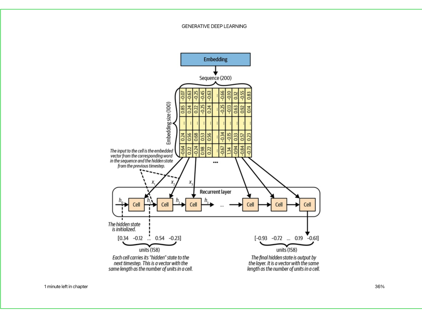
Then given an entire input sentence or sequence, you will need to represent the text as [batch_size, seq_len, embedding_size] and pad the sequences to all be the same length so that we can feed it through the model.

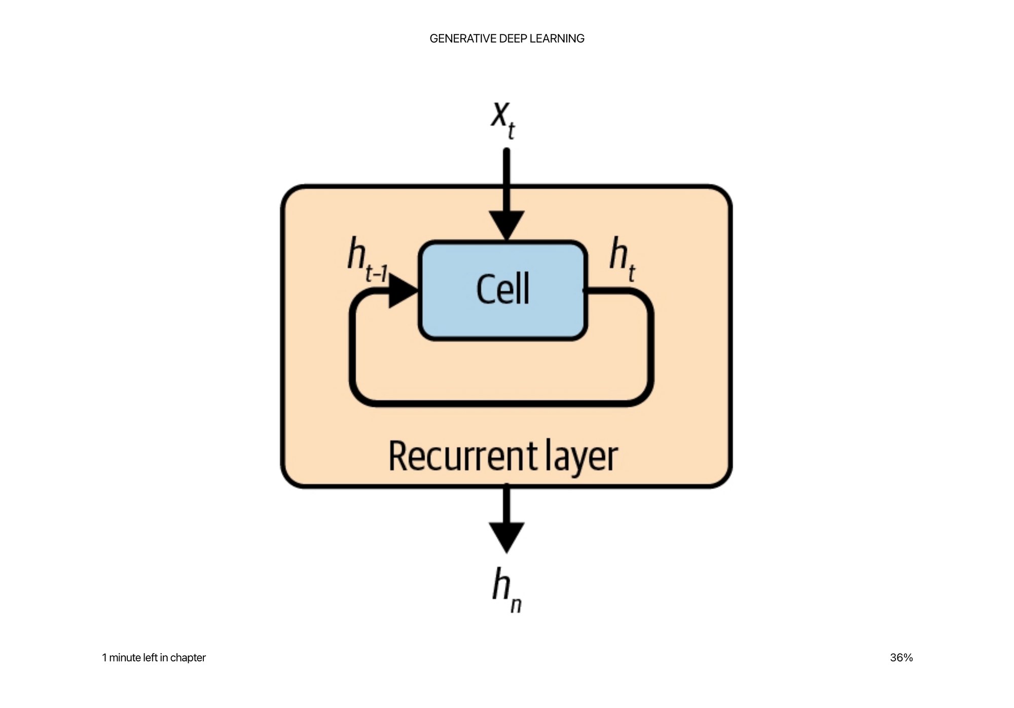
Recurrent Neural Network

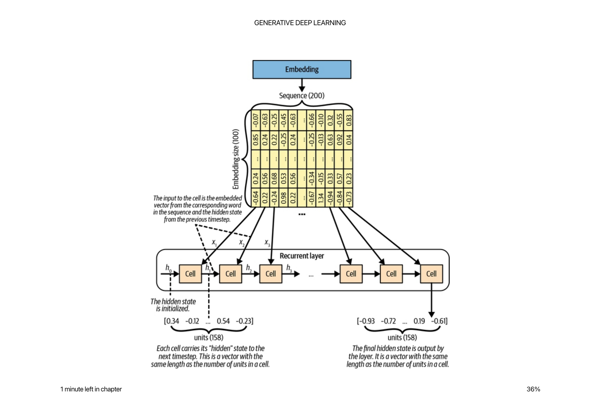
The inputs and outputs to the cell at each time step are called hidden states and are updated as you go along the sequence.

The cell actually shares the same weights along each time step, so is the same as representing it as this picture.

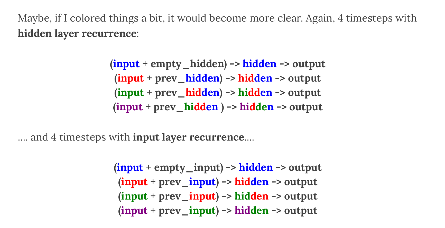
I remember liking this example explanation. https://iamtrask.github.io/2015/11/15/anyone-can-code-lstm/

The LSTM Cell

The LSTM cell takes in the current word embedding and the previous hidden state to generate a new hidden state. Internal to the LSTM cell are a few mechanisms to help identify what should be kept and what should be forgotten when generating the new hidden state.

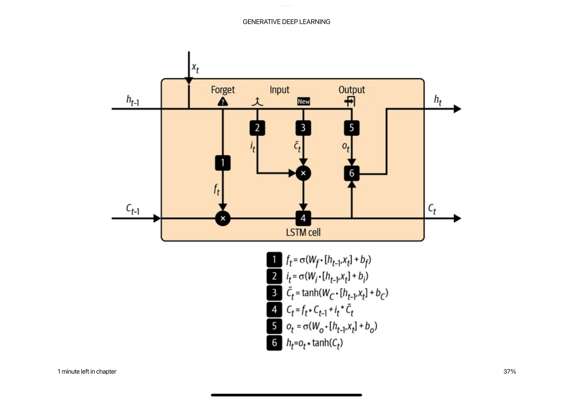
The first gate is the forget gate that is simply a linear layer with a sigmoid activation that puts the values between zero and one. This is supposed to act as a filter for information from the previous hidden state and current word embedding.

The second gate is an input gate that is similar function to the forget gate but determines how much will get added to the cells previous internal state.

The output gate takes the cell internal state and determines how much information it wants to pass on to the output.

To generate new text from the LSTM, you feed the network some existing words, and ask it to generate the next word. Then for each prediction, you feed that back in and generate the next. Instead of taking the top predicted word each time, you can add a temperature parameter that samples from the distribution. Zero temperature means the word with the highest probability is more likely to be chosen.

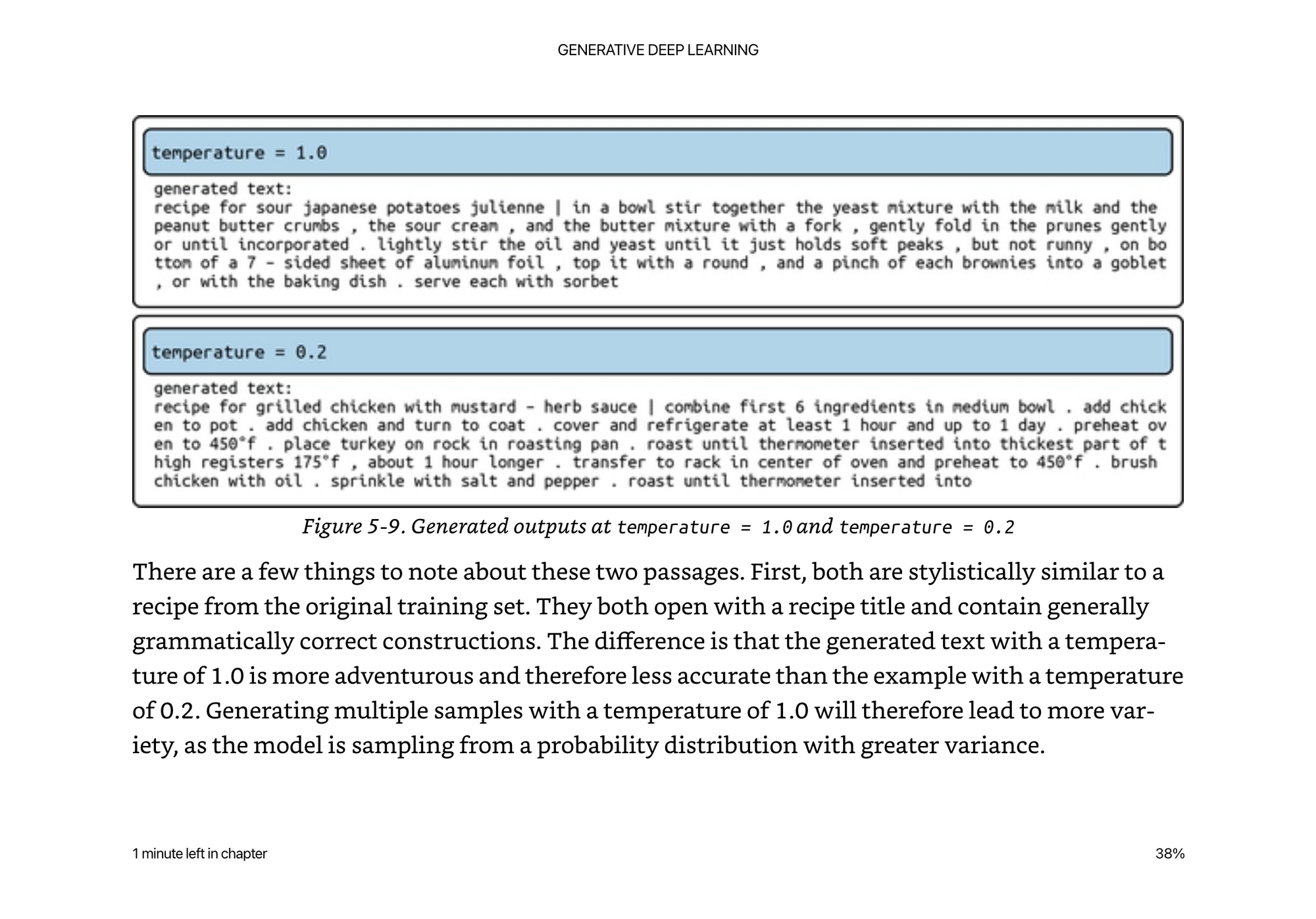
While our basic LSTM model is doing a great job at generating realistic text, it is clear that it still struggles to grasp some of the semantic meaning of the words that it is generating. It introduces ingredients that are not likely to work well together (for example, sour Japanese potatoes, pecan crumbs, and sorbet)!

We will see later that the transformer model helps solve this problem with an attention mechanism that is able to take in the full surrounding context to better generate words with better semantics and not just syntactically correct.

There are a few extensions to make recurrent networks and LSTMs a little more powerful.

1. Stacking the cells, so that each cell can pass on a higher level representation to the next cell
2. Changing the internals of the LSTM to have less filters -> GRU
3. Bidirectional RNNs where you go from front to back and back to front to help not lose information along the way.

PixelCNN

In 2016 the work done on PixelCNN showed that you could auto regressively generate images by generating the next pixel in an image by looking at the previous pixels.

Two big concepts from the PixelCNN were: Masked Convolutional Layers and Residual Blocks

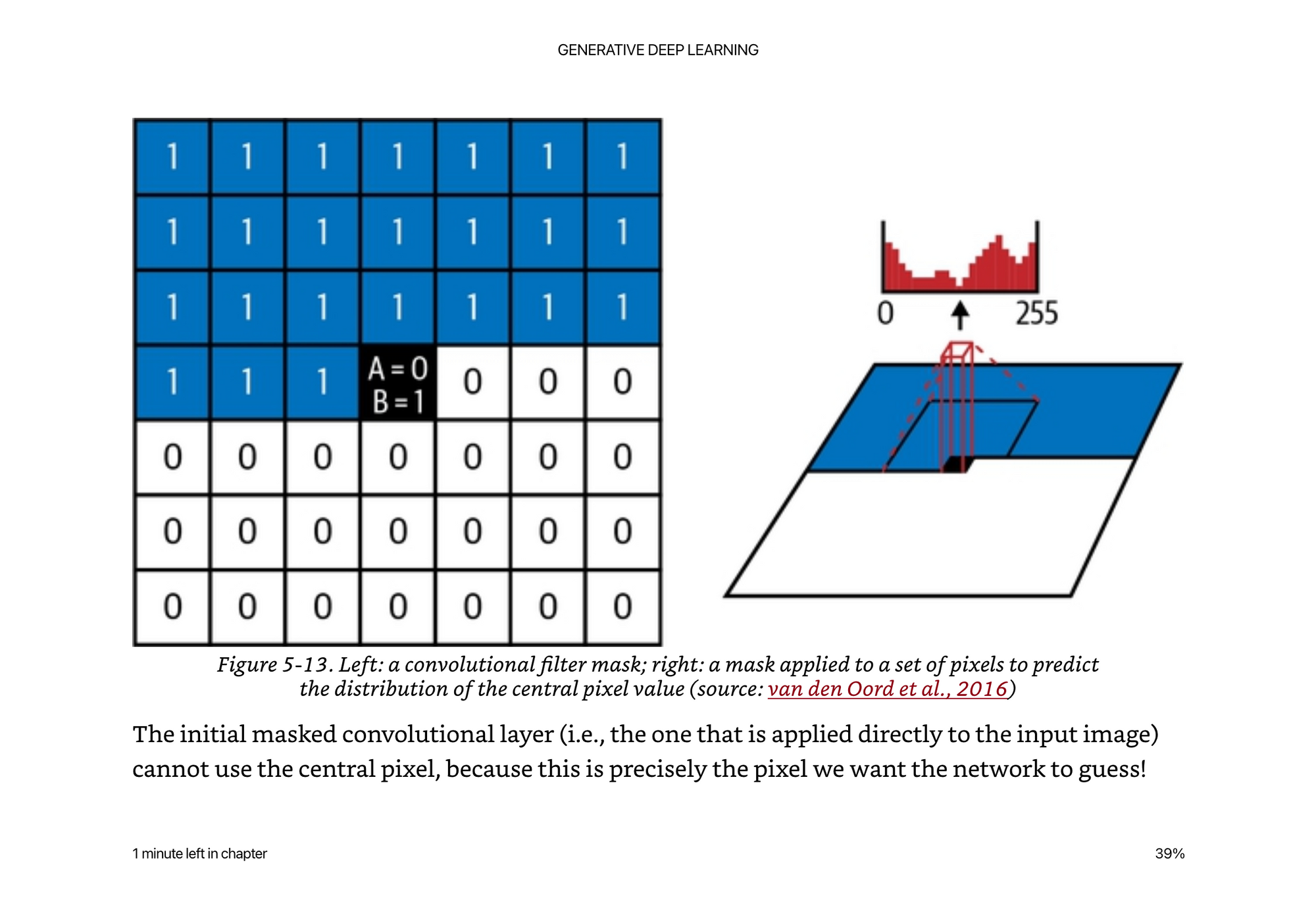
Masked Convolutional Layers

The idea behind a masked convolution is simply that we cannot use regular convolutions because they have no sense of “sequence order” of the pixels in the image. We can define order from top left to bottom right by organizing the filter mask as such.

Regular convolutions with no mask would also would show the network information about the surrounding pixels that would not make it autoregressive because we don’t know the next pixels yet in a generation context.

Residual Blocks

Residual blocks can be thought of as ways to propagate information up through the network so that it does not get “lost” or transformed too heavily in previous layers.

To do this, the output is added to the input before being passed on to the rest of the network. In other words, the input has a fast-track route to the output, without having to go through the intermediate layers—this is called a skip connection. The rationale behind including a skip connection is that if the optimal transformation is just to keep the input the same, this can be achieved by simply zeroing the weights of the intermediate layers.

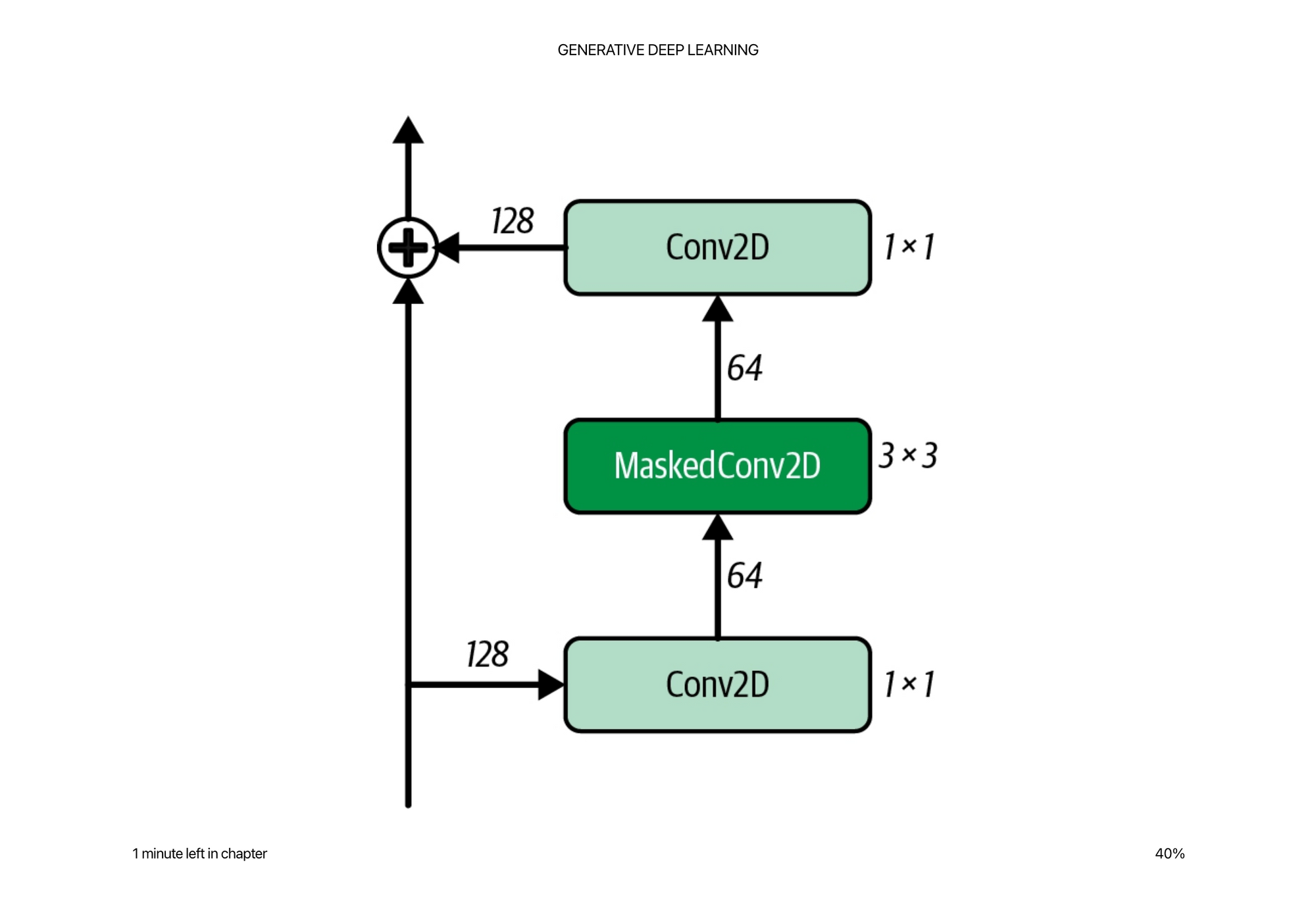
This technique is not solely used in PixelCNNs but is broadly applicable for many architectures. The core idea being, if we really need to keep information consistent or have some sort of identity transform within the network, it is useful to be able to refer to the input at every layer of abstraction.

PixelCNNs are slow to train, and slow to run inference from, because

1. They have to run a softmax over 256 values for each pixel output value, and softmax categorization does not necessarily guarantee that 201 is close to or related to 202 (which they are in image land), so it makes it harder for the network to learn this instead of encoding it somehow in the task.
2. Since you have to wait for the previous pixels to generate the next pixel, it is also slow to run inference depending on the size of the image. For example for a 32x32 grayscale image, this requires 1024 predictions sequentially to generate an image, rather than one prediction like a VAE.

That being said, the quality of results is much less blurry than the VAE, and can draw very distinct boundaries around the outputs.

Later they will cover different autoregressive models that produce even more state of the art results, but the speed of inference is definitely a price you pay with these models.

I wish he added a little more intuition around WHY they think this works better. Part of it is definitely the objective function of categorically predicting each pixel value, given previous pixel values. This replaces the more blurry mean squared error style loss you see in a VAE, and you don’t have to do as many tricks like a GAN in terms of an objective function. Pretty amazing that it works at all.

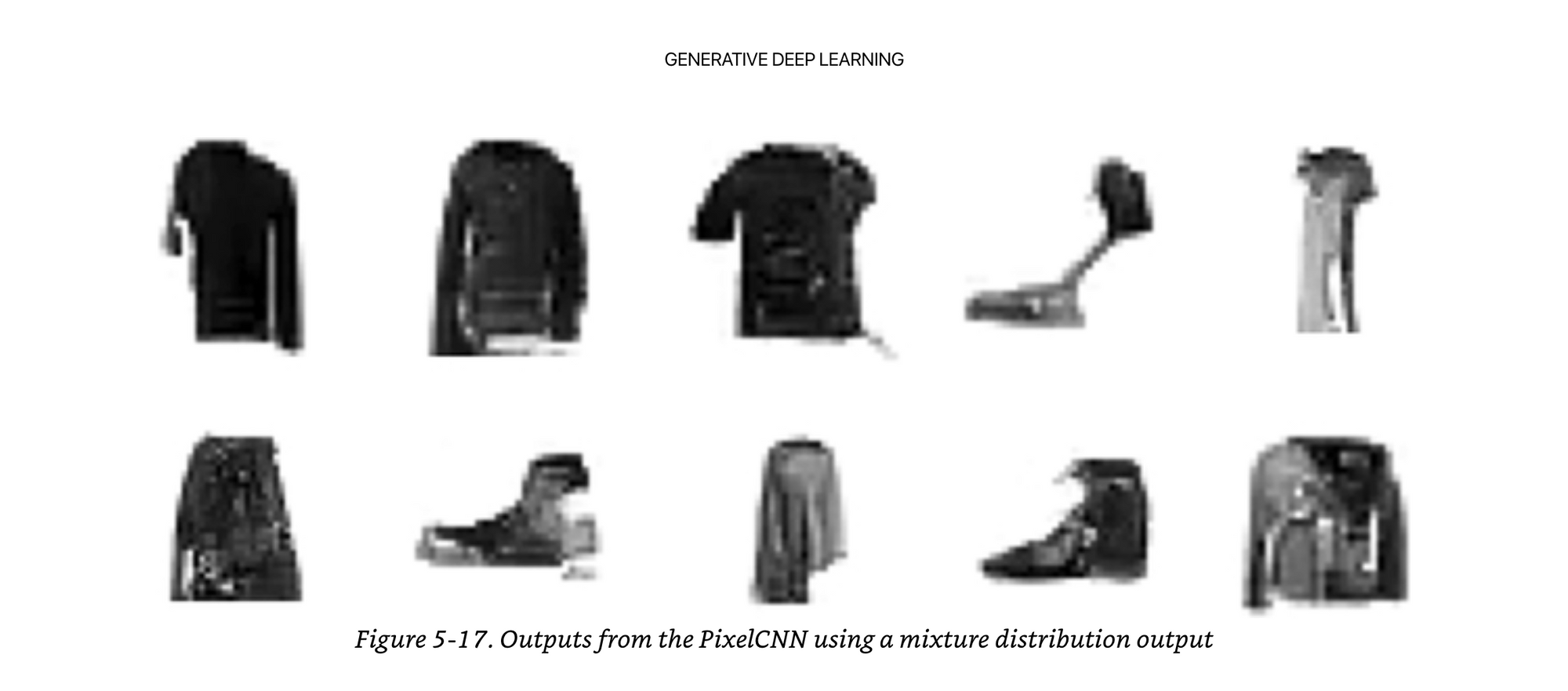
In order to speed up some of the inference, they bucket pixels into 4 pixel levels instead of 256. You can kind of see this in the artifacts above in the fashion mnist images. There are only really 4 distinct values it is producing (which if placed well, actually look pretty good).

This is far from ideal for more real world color images. To get around this they introduce a mixture distribution.

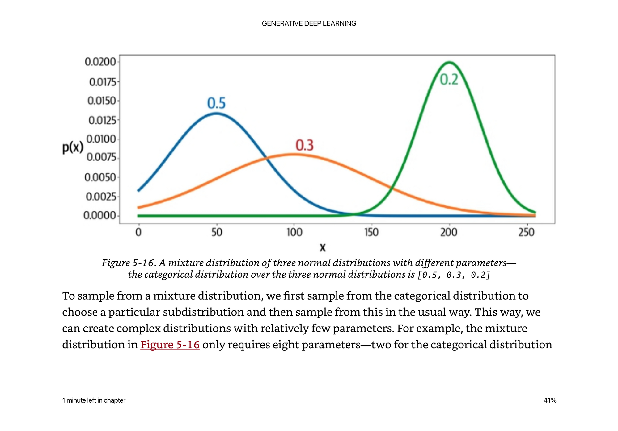
The idea here is we can learn the mean and variance of couple different normal distributions about the data, and then first sample from the categorical distribution, then sample from the distributions with different mean and variances depending on the categorical distribution. Now we’ve only added 8 parameters, but can get a more smooth set of output values.