Join the Oxen.ai "Nerd Herd"

Every Friday at Oxen.ai we host a public paper club called "Arxiv Dives" to make us smarter Oxen 🐂 🧠. These are the notes from the group session for reference. If you would like to join us live, sign up here.

The first book we are going through is Generative Deep Learning: Teaching Machines To Paint, Write, Compose, and Play.

Unfortunately, we didn't record this session, but still wanted to document it. If some of the sentences or thoughts below feel incomplete, that is because they were covered in more depth in a live walk through, and this is meant to be more of a reference for later. Please purchase the full book here, and join live for future sessions.

Generative Hello World

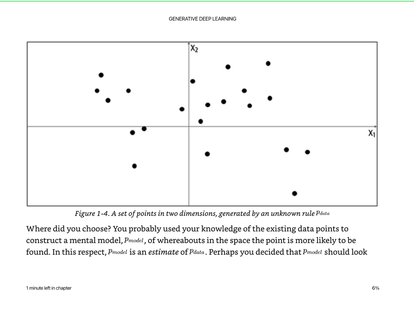
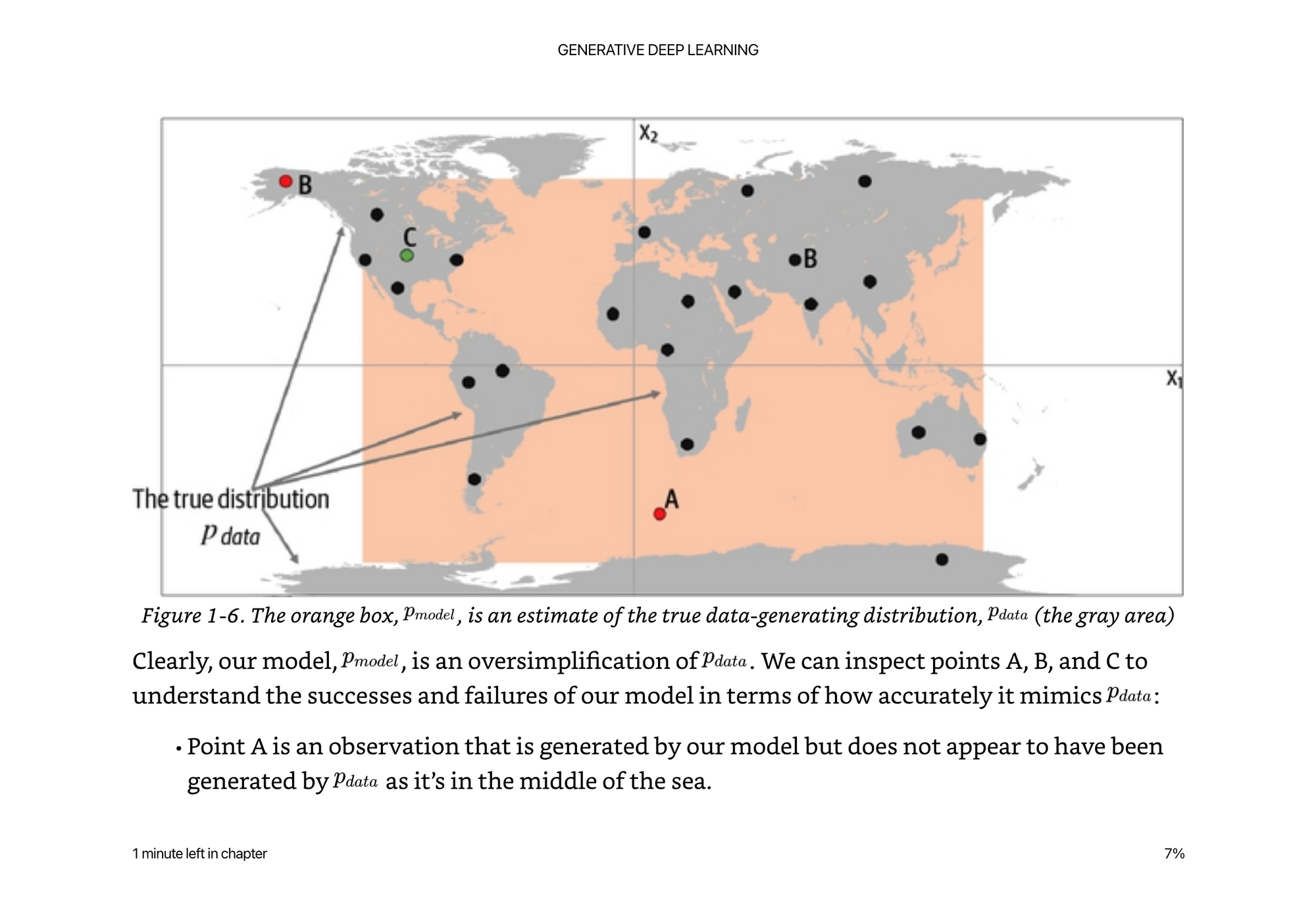
P(x) = P(x1, x2)

Can we tell what this distribution is?

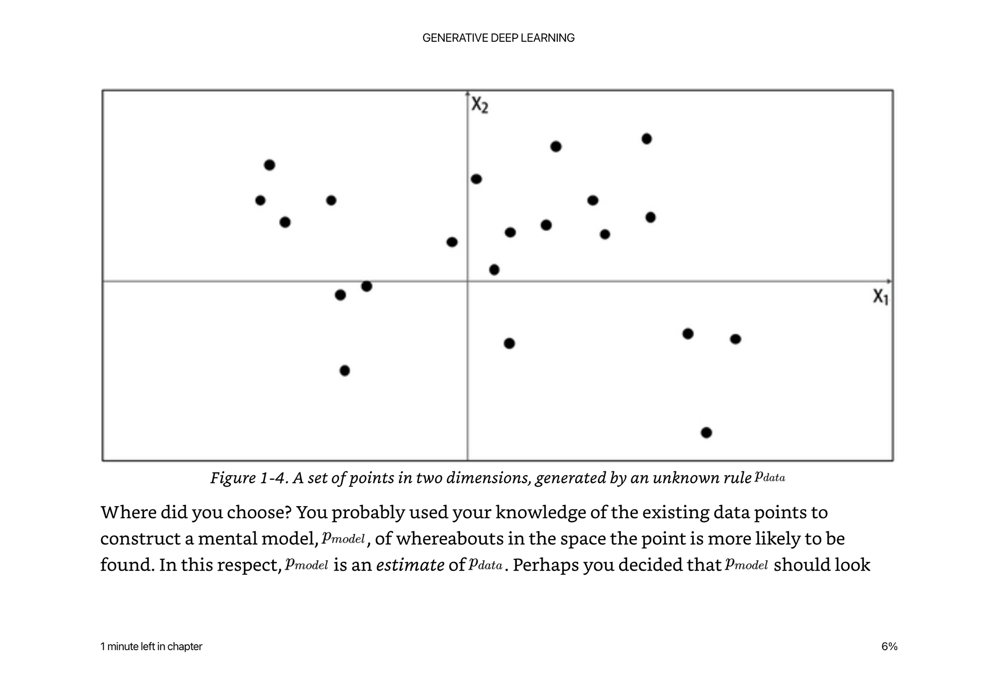
Hint: It is actually something from the real world, but we don't have enough data points to tell.

If we chose a simple model, of anything within the bounding box of x,y,width,height we would be wrong.

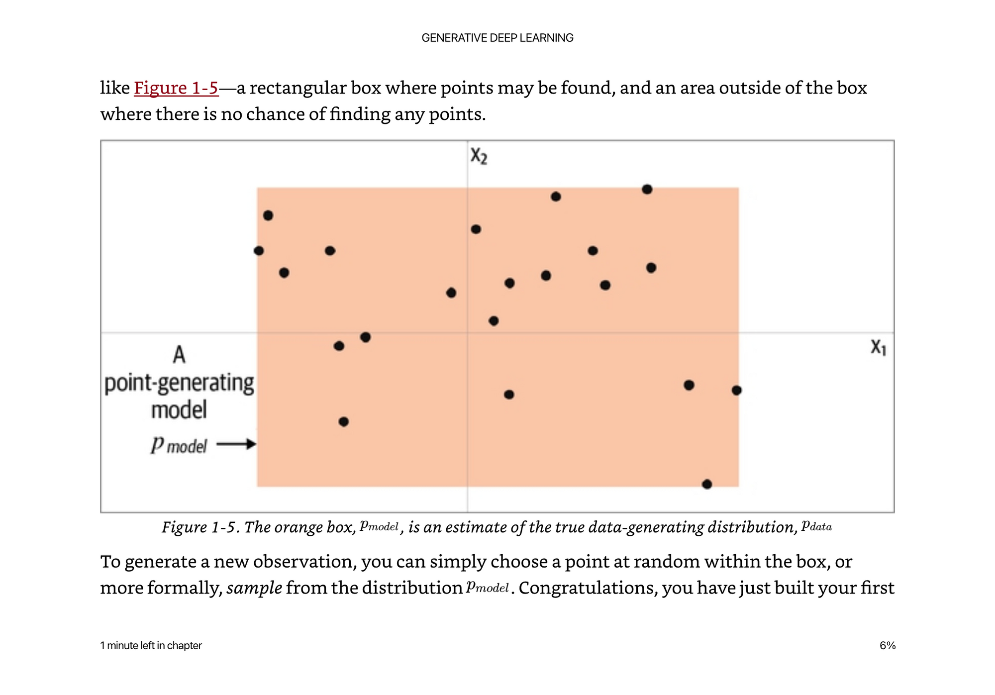
The real distribution is much more complex, yet we do not have many data points, so it is hard for us to model. The probability of the model being x,y,width,height is a simplification of the data. Above is a simple uniform distribution over the orange box.

The real data points are actually from landmasses on an image of the world. If we were trying to train a model to distinguish between land and water masses, we would be very wrong by choosing a rectangle to model it.

Representation Learning (Features)

When asking someone to draw a picture of you, they wouldn’t start with asking “what color is pixel 1, pixel 2, pixel 3” etc. They would ask, what color is your hair? How tall are you? Are there are distinct facial features? These high level abstractions allow us to create a lower dimensional space of features than the high dimensional space of x,y or x,y,z of every pixel of your face, and is much easier to work with.

We call this lower dimensional space the latent space which is a representation of some high dimensional observation.

If you think about writing a program to calculate the volume of a cylinder. You actually only need two variables in the latent space: radius and height. This is much more efficient that storing every single atom in space to represent the volume.

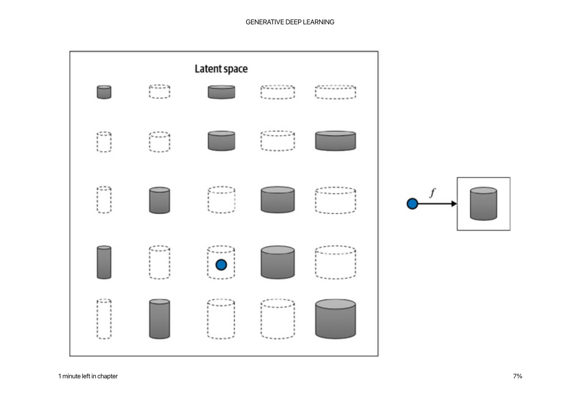
It is magical that you can distill a complex generative program down to two variables. Whenever thinking of generative modeling, it is helpful to think what features or variables are modeled in the latent space. In other words, what attributes would you describe and break down to describe this object to a computer?

It is much easier to manipulate the latent space than it is to manipulate the pixel space. There are many more pixels in an image than there are latent variables in a good generative model.

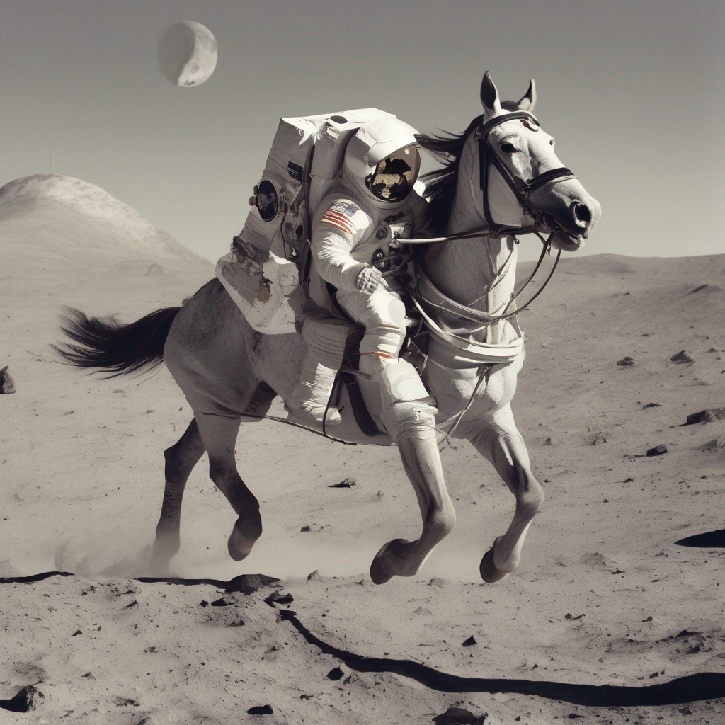
For example, in image generation, you might just tweak the latent variable that represents “height” to make a taller horse, or smaller astronaut, rather than trying to balance each pixel of each leg, etc.

The concept of encoding the training data into a latent space is a core concept of generative modeling. The problem is, unlike the cylinder, sometimes it is hard and complex to find what the variables are, and how they interplay with each other. To make a taller horse, it is not as simple as the relationship between radius and height, there are many more variables at play with non-linear relationships.

Core Probability Theory

Terms in probability are relatively simple if you look at them one at a time, but can blow up your brain if you look at an equation without knowing each individual component. They really help read and digest research papers, but it always takes me going back to the simple version to not think the author is speaking another language.

Sample Space - The complete set of values that X could take (all of the points on land, and not in sea, in the example 2D distribution above)

Probability Density Function - A function that maps all the points in the sample space from 0-1 probability. The integral over all the points in the sample space must equal 1, so that it is a well defined probability distribution. While there is only one true probability density function, there are infinitely many density functions p_model(X) we could use to estimate p_data(X)

Parametric modeling - A parametric model is one that defines a finite set of parameters to estimate a probability density function. Parameters W. In the example above x1,x2,y1,y2 could be the most simple 4 variable function for a uniform distribution over the box.

Likelihood - L(W|x) of a parameter set W is a function that measures the plausibility of W given some observed point x. L(W|x) = pW(x). The likelihood of the weights being correct at a point x is defined as the probability density function at that point X. So you can take the product of all of the probabilities of all points X within your probability density function to get the full likelihood.

We use the log likelihood since multiplying a lot of small numbers together in a computer will run into floating point errors.

Parametric modeling is all about the optimal set of parameters that maximizes the likelihood of observing the dataset X.

Maximum likelihood estimation - finding the best set of W to explain some observed data X. Argmax(X, L(W|x)).

Neural networks often minimize loss functions so you minimize the negative log-likelihood.

Generative modeling can be thought of as maximizing the likelihood of estimating the data X given parameters W. In high dimensional space it is intractable to go over all the sets of W, so we need techniques to estimate W.

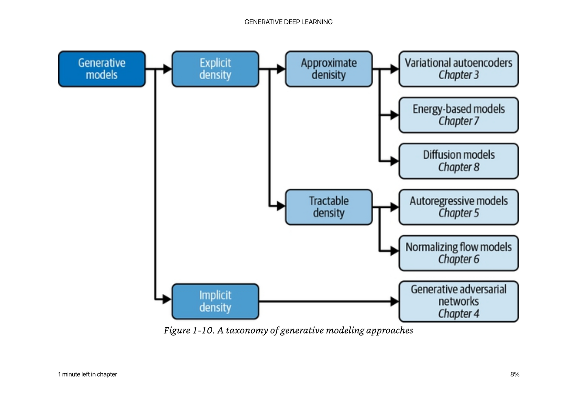
Many techniques for modeling the data X. We can approximate the probability density function. Or have a density function that is tractable to calculate. Or have an implicit density function that we are trying to model.

Machine Learning x Deep Learning

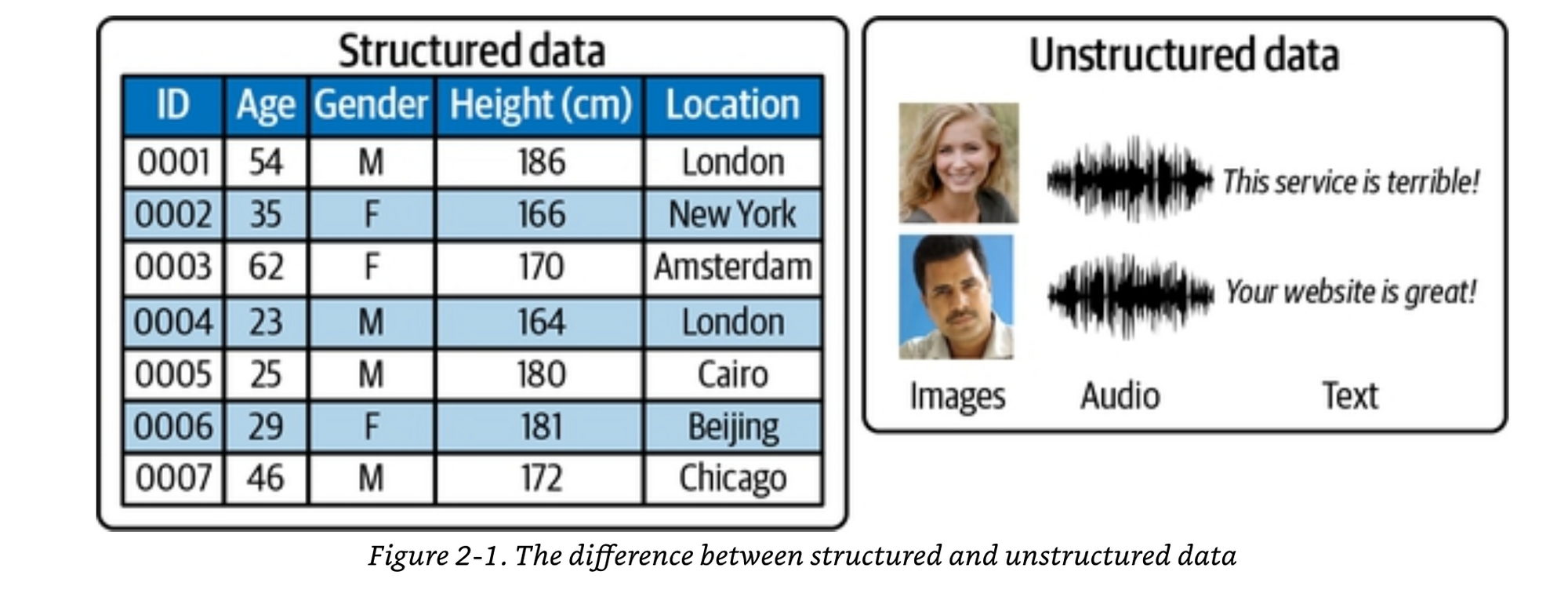
Deep learning is a class of machine learning algorithms that uses multiple stacked layers of processing units to learn high-level representations from unstructured data.

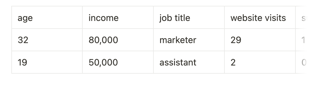
Structured data - tabular

When our data is unstructured, individual pixels, frequencies, or characters are almost entirely uninformative. For example, knowing that pixel 234 of an image is a muddy shade of brown doesn’t really help identify if the image is of a house or a dog, and knowing that character 24 of a sentence is an e doesn’t help predict if the text is about football or politics.

With unstructured data, you have to abstract the individual values to higher level features to be able to do useful operations on them.

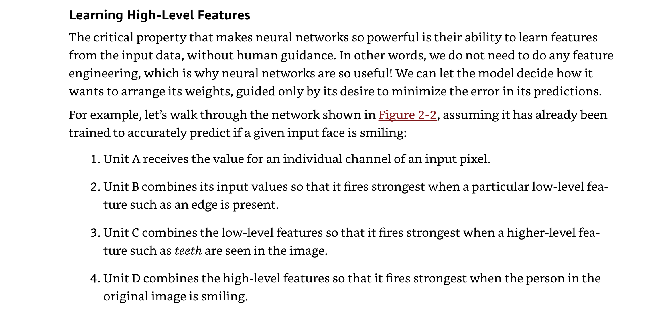
Deep neural networks help abstract the individual values (pixels, frequency, characters, etc) to higher level features (has brown hair, is smiling, has chimney, etc)

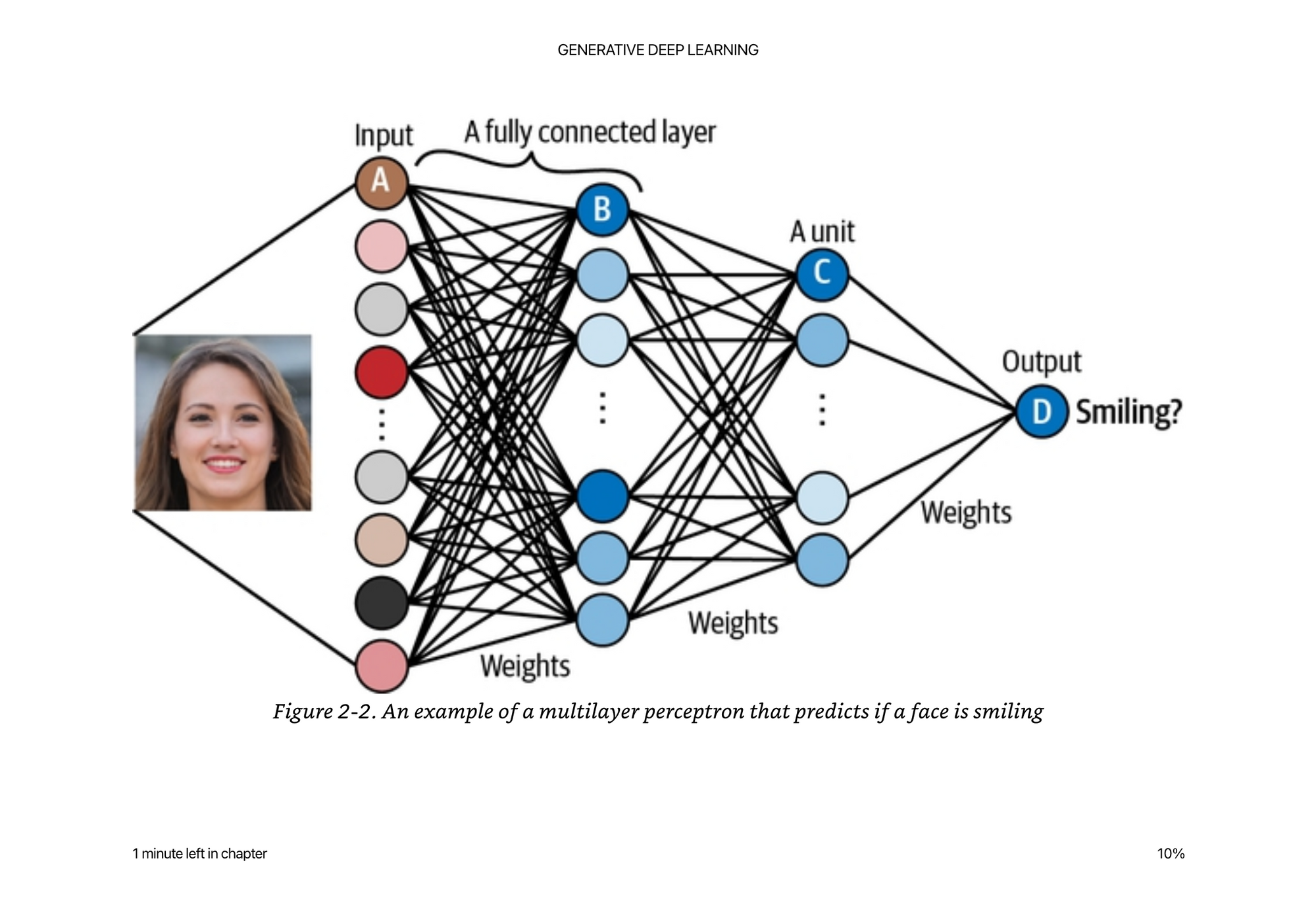
If we think about the terms above. The probability density function is the neural network, where the image is one sample in the sample space (instead of x1,x2 we have all the pixel values) and we have a function (neural network) mapping the pixel values to “is smiling?” With a value of somewhere between 0..1, that we treat as a probability.

Same thing as “on land” or “on sea” in the example above, just much more complex data transformations in between.

It is a parametric model because we have all these weights W that finite (we only have N parameters in a model, ie 175Billion in GPT3 or whatever) and when you multiple them all together, you get a probability.

We are doing maximum likelihood estimation because we are trying to find the set of weights W that when multiplied together give us probability close to 1 for all the images labeled “is smiling” and close to zero for all the images that are not smiling.

Forward pass - go through the layers, transforming the input, by multiplying the numbers together, to get a new set of numbers, that hopefully represents higher level features about the data.

The magic is, how do we find these magical set of weights W that give us high level representations of the data?

This is where “training” to learn high level abstractions comes in.

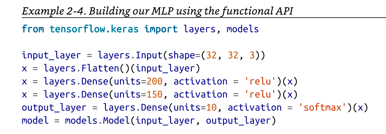
The code to define these neural networks is actually quite small.

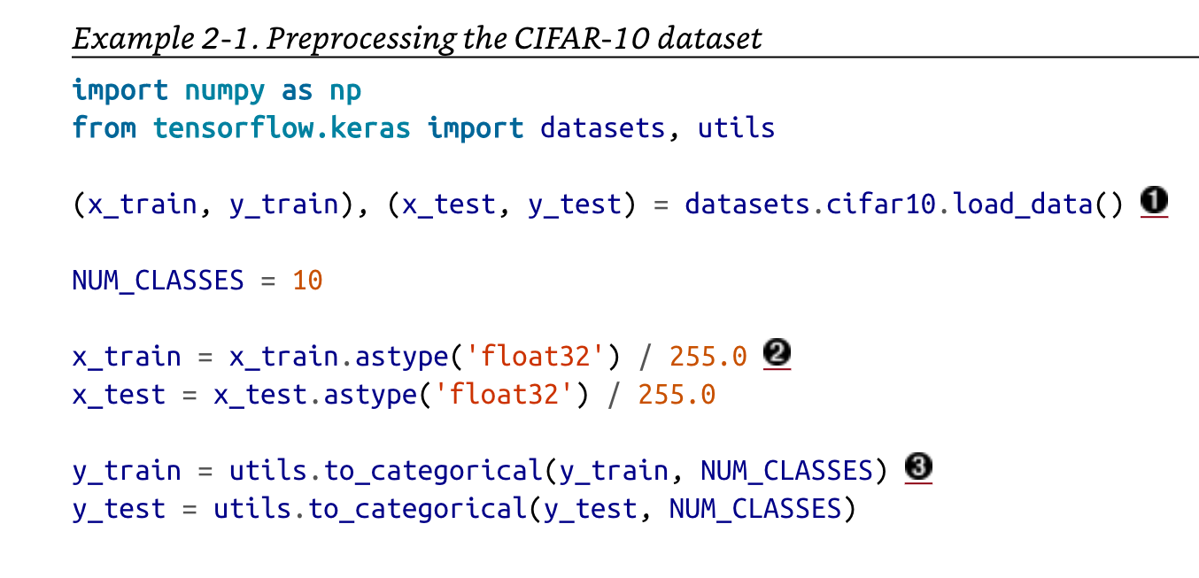
The code to load the data is actually quite small too, but has been abstracted away to download a zip file somewhere.

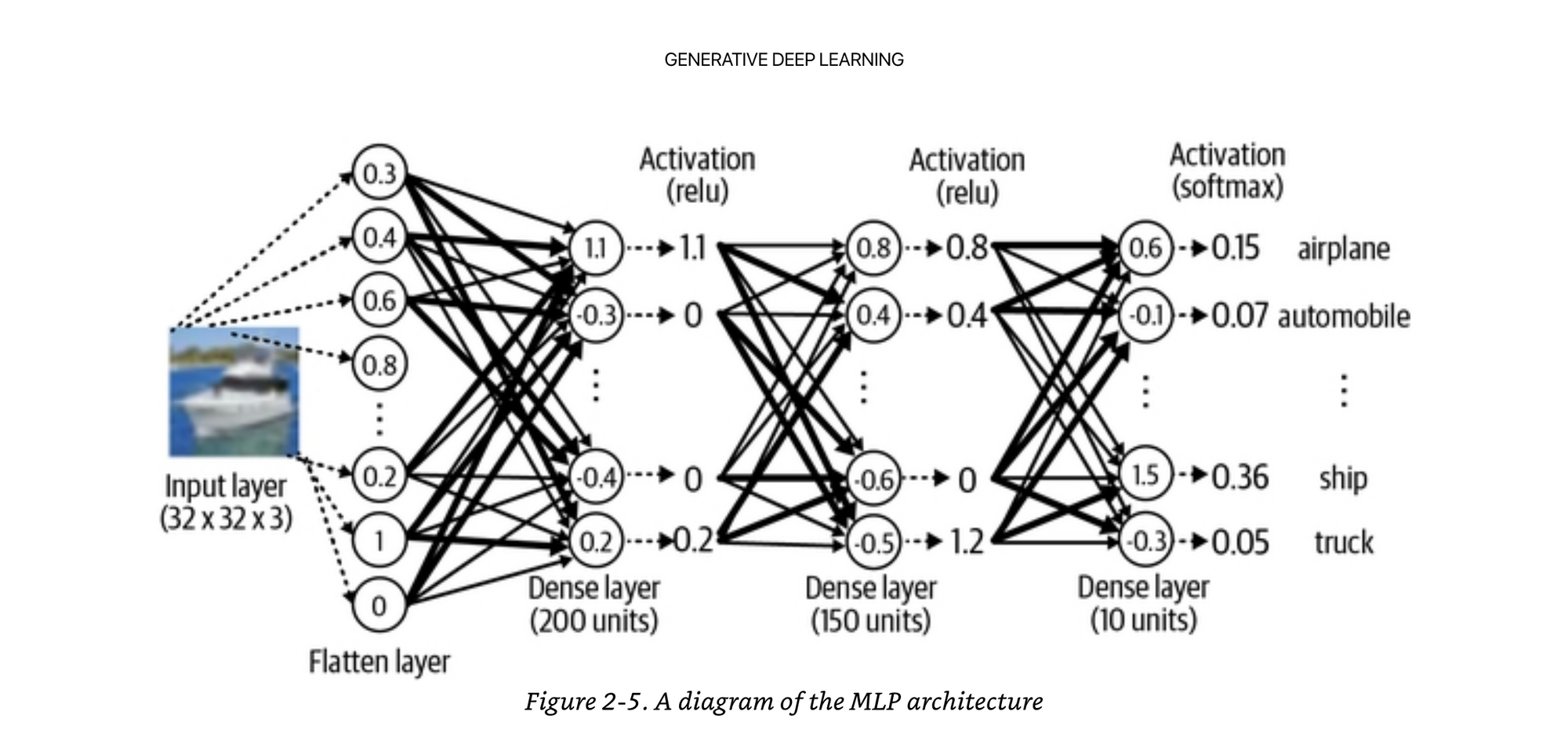
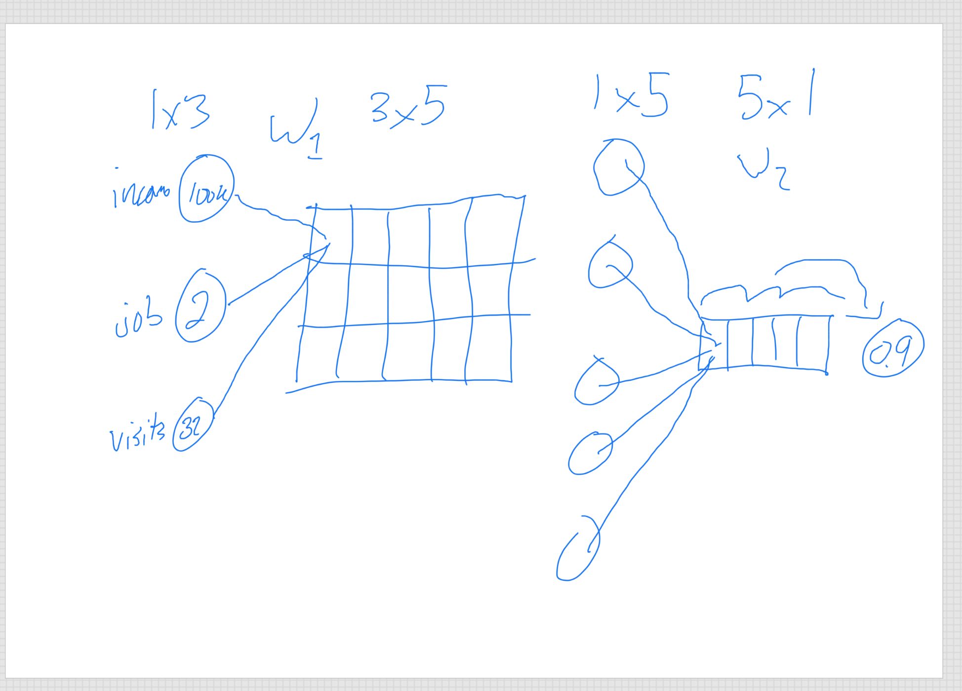
Concretely this is how the values flows through the network to classify an image.

Activation functions, linear vs non-linear. The way I like to think about these terms is if you have a linear combination of x1 * x2, you are always going to get a transformation that is a straight line between them. But what if the combination of x1 and x2 is actually a very important one.

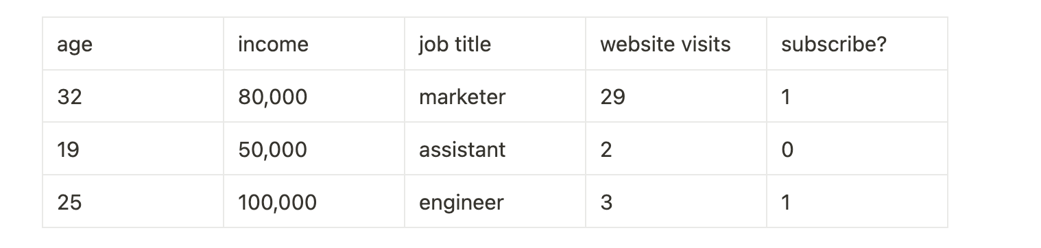
And the fact that the feature for job title is ml engineer COMBINED with number of website visits is much more important than just website visits itself is a non-linear relationship between the two variables. The more the person is an ml engineer AND they visit the website the more likely the are to subscribe. Another job could visit the site many more times and not subscribe than an ml engineer, it is not linear.

You need activation functions within a neural network so that you are not just multiplying x1*x2 in a linear fashion, you can get these exponentials that change the output non-linearly.

Loss function is simply comparing how we did to what the data tells us. Also think of it as error. There are many kinds of ways to calculate error.

Optimizer is what takes the error, and takes the weights and updates them to give us a closer approximation.

Batch Normalization is helpful to prevent exploding gradients within your network.

Exploding gradients can be caused by covariate shift. Covariate shift can be thought of as if you are carrying a giant stack of books and trying to balance, if you keep everything steady in the center, it is easy to balance, once you start overcompensating on any side it can swing back and forth until it explodes.

Batch normalization learns two parameters (scale -> gamma, shift -> beta) to keep the parameters stable based on the mean and standard deviation of the data at train time. Batch norm also has to save off the moving average of the mean and std as well as the learned parameters for test time. It’s basically a linear transform of y = gamma*x_normalized + beta. Subtract the mean and divide by the standard deviation, so that you know how much of an outlier this input is.

Dropout - Neural networks can be very good at memorizing things about the training data. This is a desirable property of learning, but can be undesirable if you can not generalize. Like memorizing answers to an exam rather than knowing the general techniques to solve a problem. Dropout helps prevent overfitting by randomly zeroing out weights that are used during training, so that the network can not be too reliant on one set of weights or another, it has to distribute and generalize the knowledge throughout it’s weights. It still has to produce accurate predictions in unfamiliar conditions.