How to Fine-Tune a FLUX.1-dev LoRA with Code, Step by Step

Greg Schoeninger

6/28/2025

FLUX.1-dev is one of the most popular open-weight models available today. Developed by Black Forest Labs, it has 12 billion parameters. The goal of this post is to provide a barebones example of the training loop to help you learn and implement your own fine-tuning pipelines.

Feel free to skip directly to the code if you already have background on the FLUX models. This code can be run directly on a GPU in a Marimo Notebook Oxen.ai. Signing up will give you $10 of free credits to get started.

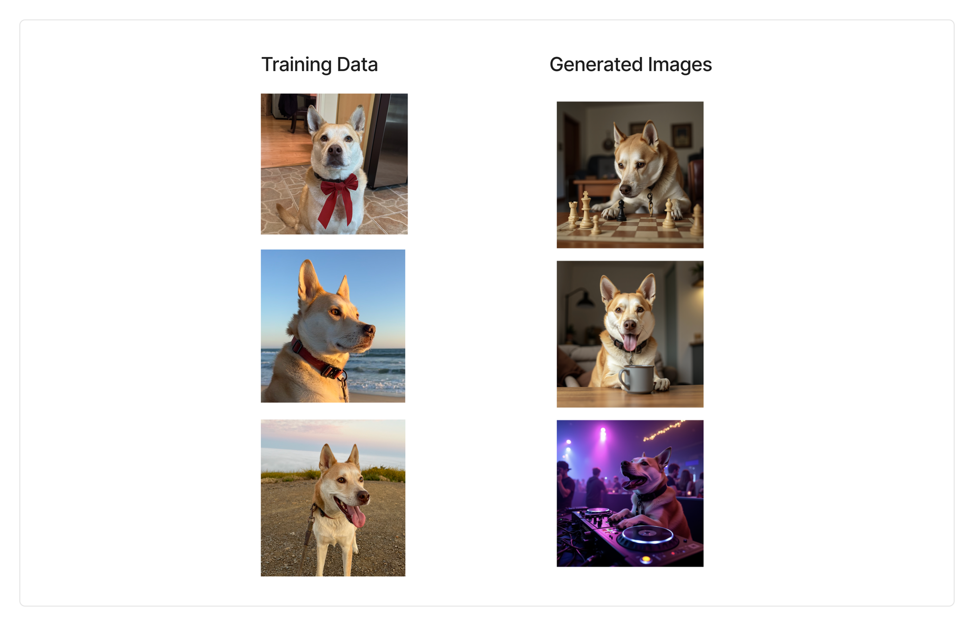
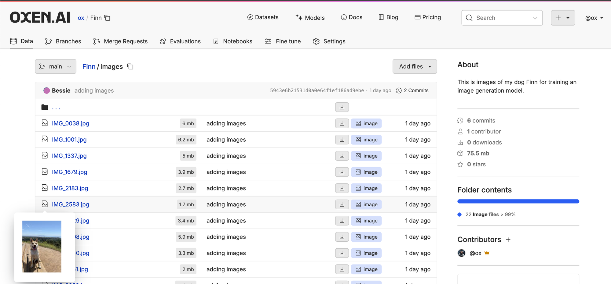
If you haven’t seen examples generated by a fine-tuned FLUX model, they are of very high quality. For example, here is a quick experiment I ran using the code below. I took 20 images of my dog from my camera roll (left column) and was able to fine-tune FLUX to generate the images on the right.

Black Forest Labs initially launched the Flux series with a few open weights models:

FLUX.1 [dev] - An open-weight, guidance-distilled model for non-commercial applications. It has similar performance to pro, but you can contact them for a commercial license.
- NOTE: This license just got a whole lot more restrictive, and is pretty expensive at $999/month
FLUX.1 [schnell] - The fastest model is tailored for local development and personal use. It is openly available under an Apache 2.0 license 🎉
- Schnell is a step distilled model, meaning it can generate an image in just a few steps. However, this makes it impossible to train on it directly because every step you train breaks down the compression more and more.

Just yesterday, they also announced the newest member of the family FLUX.1 Kontext, which is useful for editing images with text. This blog will focus on FLUX.1-dev, and we will follow up with more information on FLUX.1-Kontext with our next deep dive.

👨‍🎨 The Task

Our task is to train a LoRA on a character of our choosing. LoRAs are a smaller, lightweight set of parameters that are fast to train and can give a model superpowers. They can be used to customize models and imbue them with new characters or styles. In this case, we will be using my dog.

The two most common questions I get when diving into fine-tuning are:

How much data do I need?
How do I get the data?

For this example, all we needed was 20 diverse images of my dog. As a general rule of thumb: the more data, the better; the higher the quality, the better; and the more diverse the data, the better.

As for data sourcing, we will be doing a follow up post on how to generate synthetic data from existing frontier models. If all it takes is 20-100 images, it is worth doing some hand capture from your team or hiring with the skills to collect the initial images.

🧠 The Model

Before we dive headfirst into the code, it's helpful to have some background on the model we're training. There's a lot of jargon in the component names, and understanding the architecture will help you grasp the internals more clearly.

From the FLUX.1-Kontext paper the team states that: FLUX.1 is a rectified flow transformer trained in the latent space of an image autoencoder. Let’s break down the two most important terms “image autoencoder” and “rectified flow transformer”.

Autoencoder

Let’s start with what is an autoencoder? An autoencoder takes in an image, and compresses it down to a vector through a model such as a convolutional neural network, then decompresses it trying to reconstruct the original image from only the vector (z). This intermediate vector is what is called the “latent space” representation of the image.

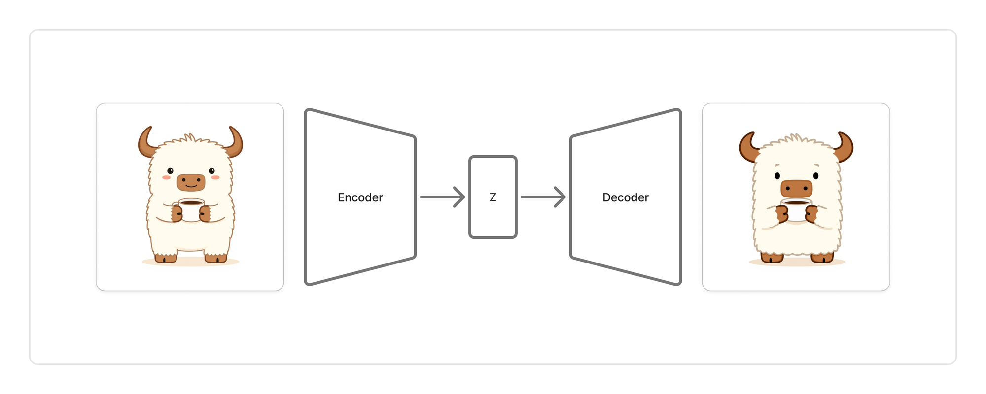
Having a good representation of the image in latent space is key for many aspects of the diffusion process. Autoencoders are also really easy to train since they don't need any human labeled images. They are essentially using the identity function as the objective.

Rectified Flow Transformer

The rectified flow transformer was introduced in the “Scaling Rectified Flow Transformers for High-Resolution Image Synthesis” paper, otherwise known as Stable Diffusion 3.

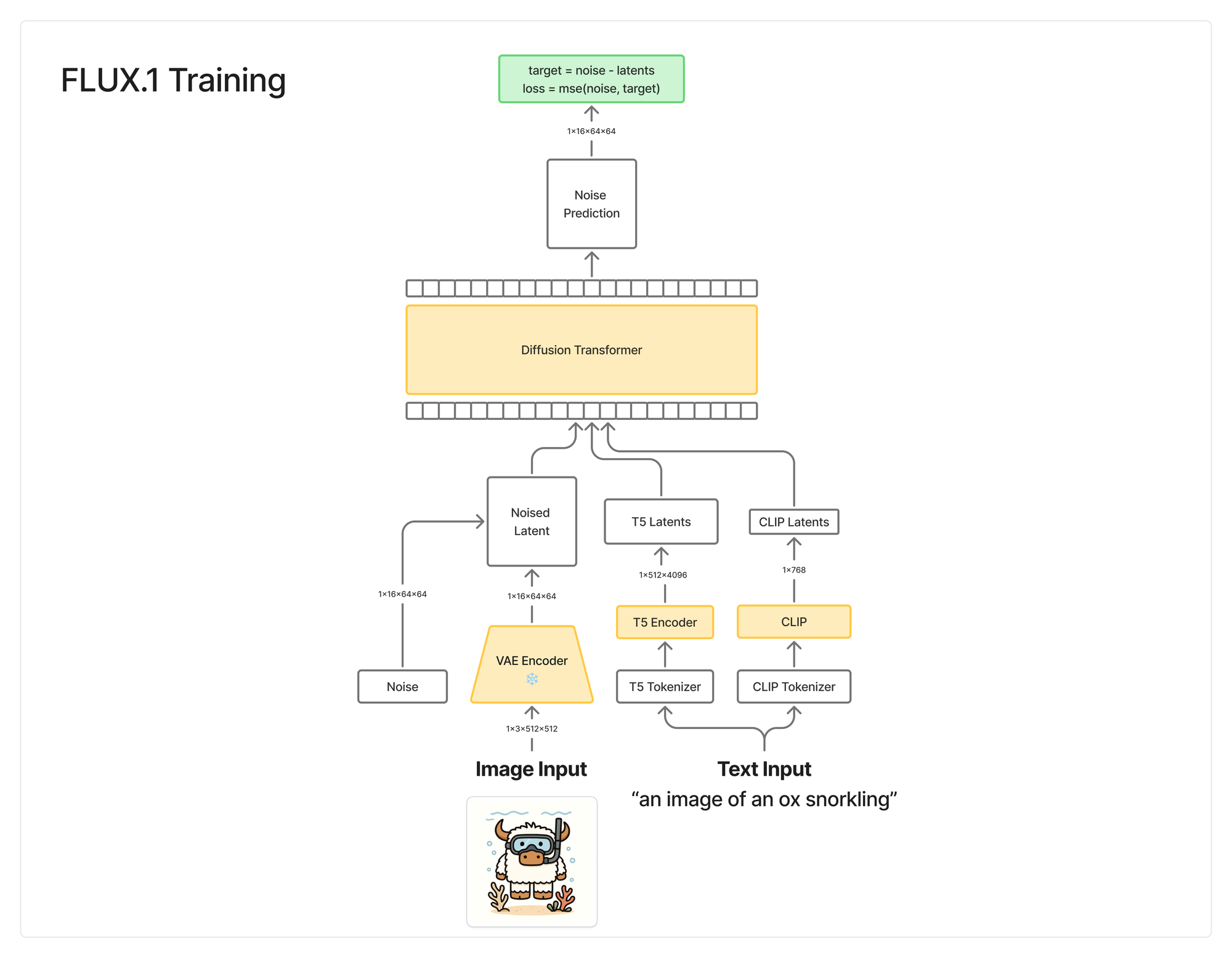
The diagram below abstracts all the internals of the Diffusion Transformer, but will give you a sense of the moving parts during training. We will reference these parts while implementing the code. If you are unfamiliar with Diffusion Models, we have a few Arxiv Dives on the process that will clear up some of the terminology.

The most important parts to pay attention to are:

VAE - Encode the image into latent space
T5 Encoder - Encode the text into latent space
CLIP - Encode the text into latent space
Noise - What we are trying to remove from the image. This is where the "rectified flow" comes in.
Diffusion Transformer - Process the latent space to predict the noise
Loss function - How close the noise prediction is to the actual noise

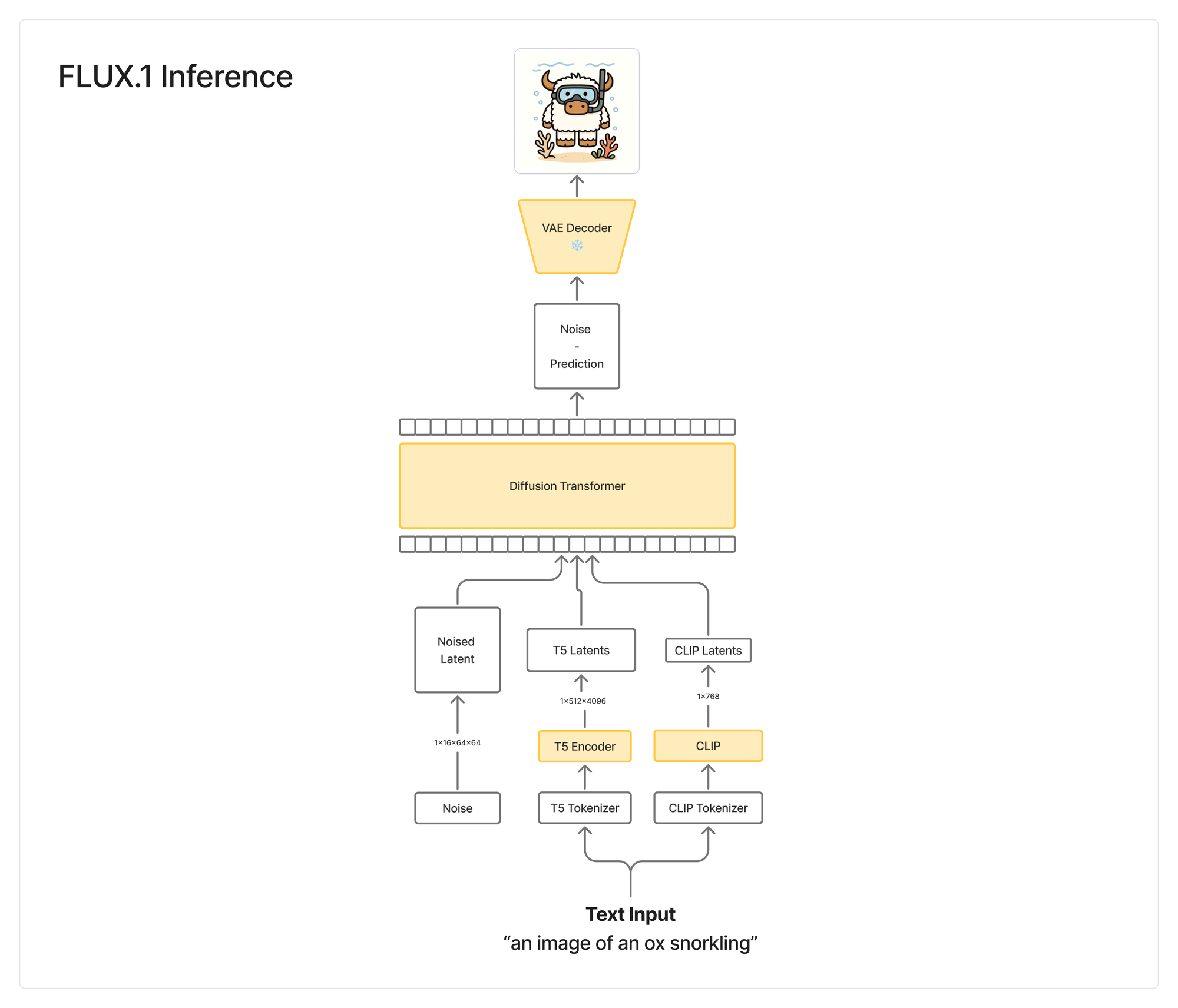
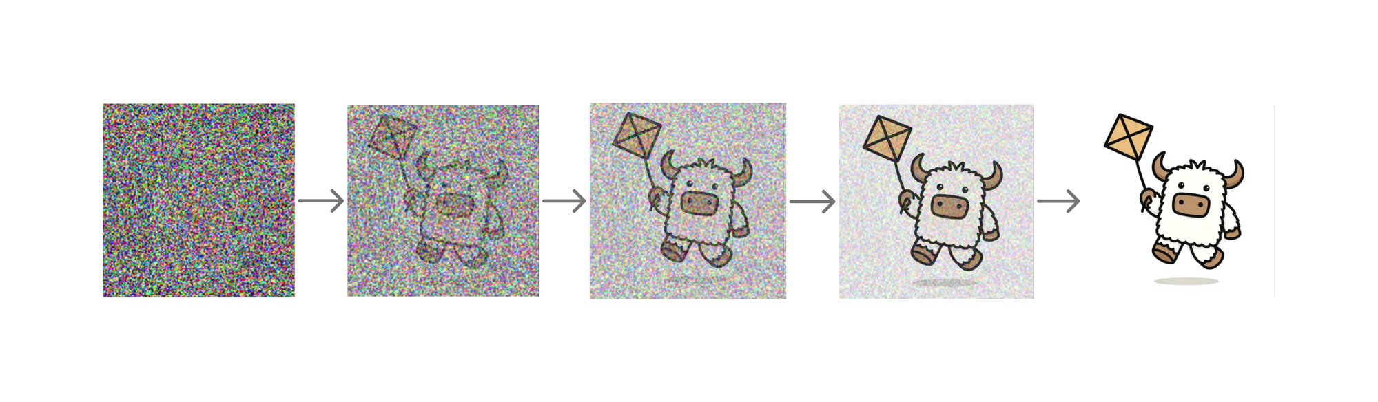
After training, you no longer have the image input + VAE encoder. We simply input the text and the noise. You then use the VAE decoder to decode the noise, remove the predicted noise, and iterate N times until you have a valid image.

💻 The Hardware

All the experiments here were run on a single H100 on Oxen.ai. These days it is pretty cheap and easy to rent an H100 in the cloud for a couple hours, so I didn’t optimize for anything smaller. In theory you can quantize the model and train it on an A10 with 24GB of VRAM, but I wanted a dead simple example without many bells and whistles.

👨‍💻 The Code

We will be writing all of the code in a Marimo notebook, which will make it easy for us to iteratively run the cells and poke around the data and model. Marimo notebooks are pure Python, and can also be run as command line applications or web apps making it easy run anywhere.

Feel free to grab this file and run it on a GPU in your own Oxen.ai repository.

⚙️ Install Dependencies

The code needs the following dependencies installed.

pip install pandas
pip install torch
pip install datasets
pip install trl
pip install peft
pip install huggingface_hub[hf_transfer]
pip install torch
pip install torchvision
pip install pillow
pip install tqdm
pip install diffusers
pip install transformers
pip install protobuf
pip install sentencepiece
pip install einops
pip install bitsandbytes
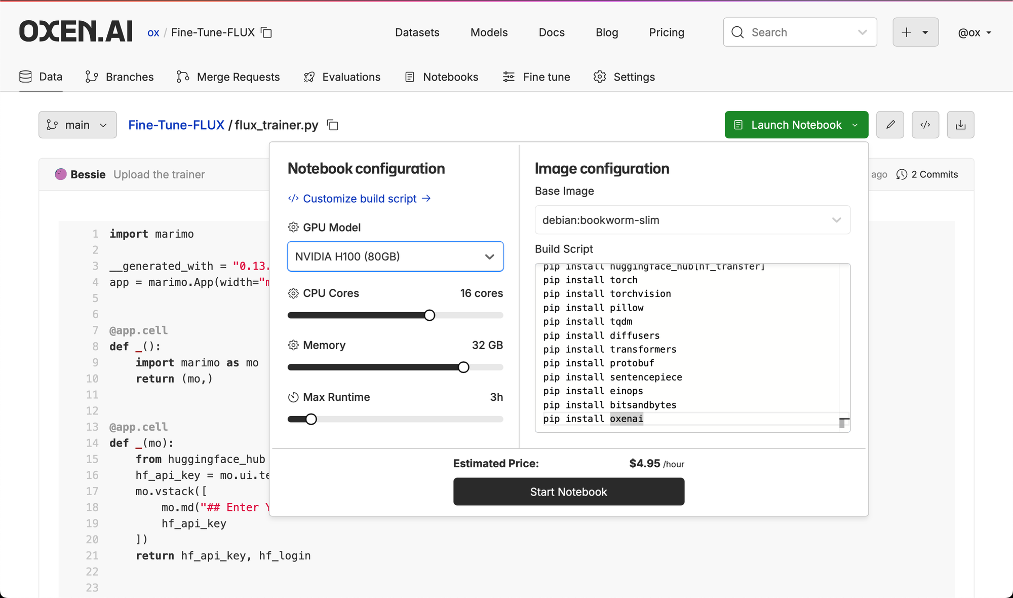
pip install oxenai

When running in Oxen.ai, simply upload your file, click "Launch Notebook", and provide your dependencies in the custom build script. Be sure to select a beefy GPU like the H100 with enough memory.

👨‍💻 Import Dependencies

In the first cell of the Notebook, start by importing all the libraries that we will need for training.

# Generic libs
import os
import math
import random
import gc
import json
from pathlib import Path
from datetime import datetime
from tqdm import tqdm

# Data types and utils
import torch

# For F.mse_loss
import torch.nn.functional as F

# To load the datasets
from torch.utils.data import DataLoader, Dataset
from torchvision import transforms
import numpy as np
import pandas as pd

# Loading Models
from diffusers import (
    FluxTransformer2DModel,
    FlowMatchEulerDiscreteScheduler,
    DDPMScheduler,
    AutoencoderKL,
    FluxPipeline
)
from transformers import T5TokenizerFast, T5EncoderModel, CLIPTextModel, CLIPTokenizer
from peft import LoraConfig, get_peft_model, TaskType, get_peft_model_state_dict
from einops import rearrange, repeat
import bitsandbytes as bnb

# Saving Data to Disk
from safetensors.torch import save_file
from PIL import Image

# Saving Data to Oxen.ai (optional)
from oxen import RemoteRepo

We will be saving the training data, samples during training, and model weights to an Oxen.ai repository, hence the oxen dependency at the end. This is optional, but a good way to version and store your data as you are training models.

⬇️ Downloading Models

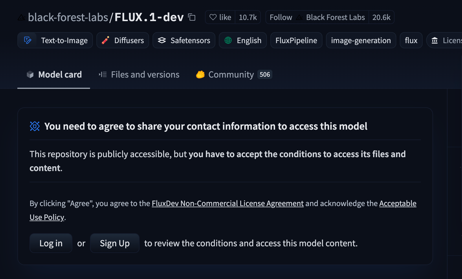
All of the initial model weights will be downloaded from black-forest-labs/FLUX.1-dev Hugging Face repository. You will need to accept the terms and conditions to access the files.

Once you have logged in and accepted the terms, click on the Files and Versions tab to understand what we are about to download. Each of the underlying model weights are stored in a separate folder that needs to be specified when loading the model.

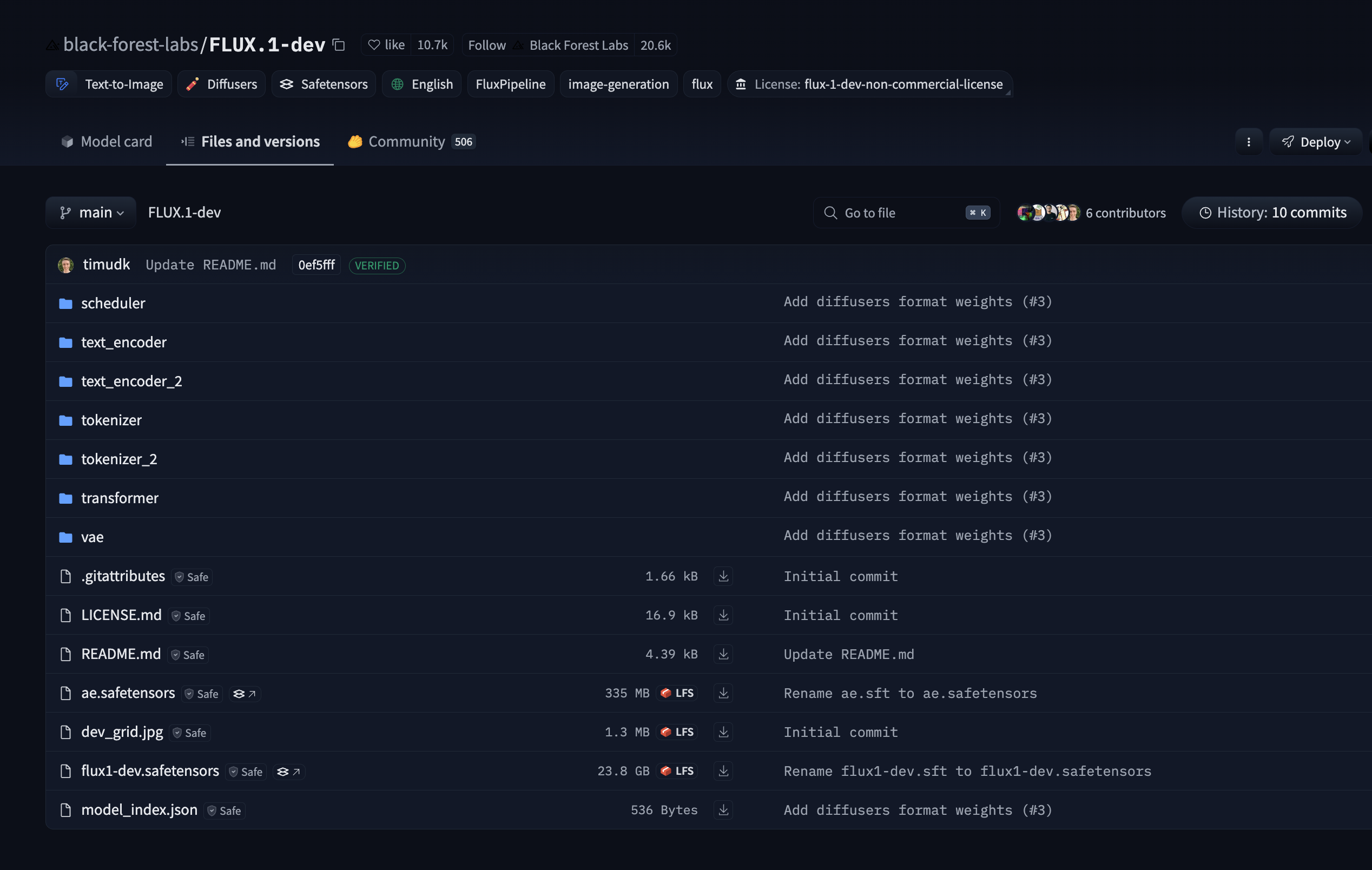
In our next Notebook cell, let's write a function to download the different components of the model. The main classes we will use to download the weights are FluxTransformer2DModel, AutoencoderKL, CLIPTextModel, CLIPTokenizer, T5EncoderModel, T5TokenizerFast. Note we pass in the subfolder to each one of them to specify where the weights live in the hugging face repository.

Let's start with the core Diffusion Transformer itself.

from huggingface_hub import login as hf_login

# Must login to Hugging Face to download the weights
hf_login("YOUR_API_KEY")

# https://huggingface.co/black-forest-labs/FLUX.1-dev
model_name = "black-forest-labs/FLUX.1-dev"

def load_models(model_name, lora_rank=16, lora_alpha=16, dtype=torch.bfloat16, device="cuda"):
    # Transfor all the models to the GPU device at the end
    device = torch.device(device)

    # Load transformer
    print("Loading FluxTransformer2DModel")
    transformer = FluxTransformer2DModel.from_pretrained(
        model_name,
        subfolder="transformer",
        torch_dtype=dtype
    )
    # For more efficient memory usage during training
    transformer.enable_gradient_checkpointing()

    // Load rest of models below...

We enable_gradient_checkpointing() in case we are running up on GPU memory limits during training. After the transformer is loaded, we must add the LoRA parameters. We'll apply the LoRA to the query, key and value matrices, as well as the feed forward layers.

# Apply LoRA
print("Applying LoRA FluxTransformer2DModel")
# Target modules for LoRA (Flux transformer specific modules)
target_modules = [
    "to_q", "to_k", "to_v", "to_out.0",  # Attention layers
    "ff.net.0.proj", "ff.net.2",  # MLP layers
    "proj_out"  # Output projection
]
lora_config = LoraConfig(
    r=lora_rank,
    lora_alpha=lora_alpha,
    target_modules=target_modules,
    lora_dropout=0.0,
    bias="none",
)
transformer = get_peft_model(transformer, lora_config)
transformer.print_trainable_parameters()

Next up is the Variational Autoencoder (VAE) to encode images to a latent space, and then decode images from a latent space. FLUX trained it's own Autoencoder, but there are other ones that could potentially be plugged in here.

# Load VAE
print("Loading AutoencoderKL")
vae = AutoencoderKL.from_pretrained(
    model_name,
    subfolder="vae",
    torch_dtype=dtype
)
vae.eval()

Next up is the CLIP tokenizer and model. This model specializes in embedding language tokens into a visual latent space.

print("Loading CLIPTextModel")
clip_encoder = CLIPTextModel.from_pretrained(
    model_name,
    subfolder="text_encoder",
    torch_dtype=dtype
)
clip_encoder.eval()

print("Loading CLIPTokenizer")
tokenizer = CLIPTokenizer.from_pretrained(
    model_name,
    subfolder="tokenizer"
)

Finally load the T5 Encoder tokenizer and model. T5 is another transformer / language model that will help encode all of the context of the sentence into a latent representation.

print("Loading T5EncoderModel")
t5_encoder = T5EncoderModel.from_pretrained(
    model_name,
    subfolder="text_encoder_2",
    torch_dtype=dtype
)
t5_encoder.eval()

print("Loading T5TokenizerFast")
t5_tokenizer = T5TokenizerFast.from_pretrained(
    model_name,
    subfolder="tokenizer_2"
)

Finally we transfer all the weights to GPU for training.

# Move models to GPU
print("Moving models to GPU")
transformer = transformer.to(device)
vae = vae.to(device)
text_encoder = text_encoder.to(device)
text_encoder_2 = text_encoder_2.to(device)

And return all 6 models as a tuple to make it easier to pass them around the code.

def load_models(model_name, lora_rank=16, lora_alpha=16, dtype=torch.bfloat16, device="cuda"):
  # Load all the models above...
  # Return all the models together
  return (transformer, vae, clip_encoder, t5_encoder, tokenizer, tokenizer_2)

Now all we need is a single line to load all the models for training.

models = load_models(model_name)

🖼️ Loading the Dataset

The dataset format we are expecting is a parquet file with two columns: image and action. The image column should contain relative paths to the images on disk. If you upload your dataset to Oxen.ai in this format, it will be easy to view, query, edit, and version.

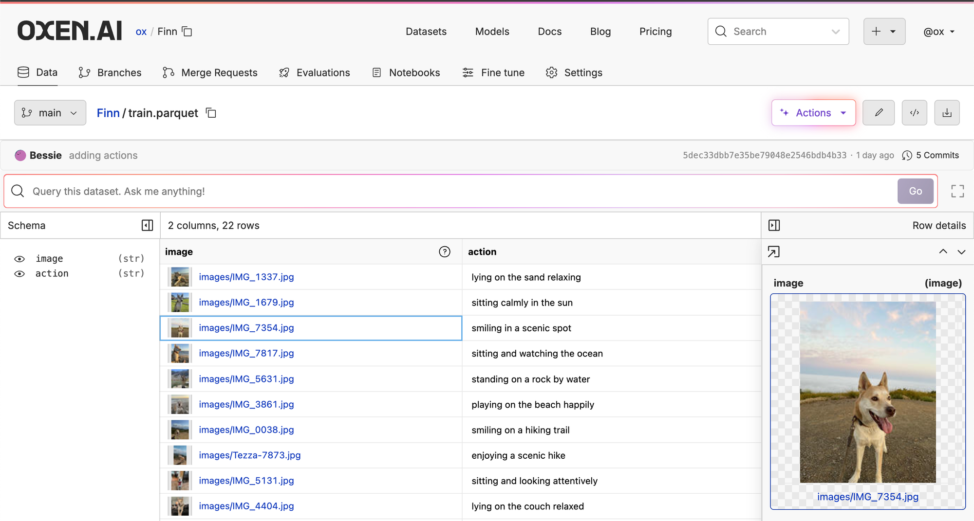
The images should be stored in a directory next to the parquet file and will be downloaded separately from the labels.

We can then subclass Dataset from pytorch to make it easy to iterate over our dataset. The important methods to implement are the __len__ to determine the number of examples and the __getitem__ method to get an individual example. Take a look at the Datasets/DataLoaders documentation from pytorch for more information.

class FluxDataset(Dataset):
    """Dataset for loading images and captions for Flux training"""

    def __init__(self, dataset_repo, dataset_path, images_path, resolutions=[512, 768, 1024], trigger_phrase=None):
        self.repo = RemoteRepo(dataset_repo)
        self.resolutions = resolutions
        self.trigger_phrase = trigger_phrase
        self.images_path = images_path

        if not os.path.exists(images_path):
            print("Downloading images")
            self.repo.download(images_path)

        if not os.path.exists(dataset_path):
            print("Downloading dataset")
            self.repo.download(dataset_path)

        # Load the dataset
        df = pd.read_parquet(dataset_path)

        # Read all images and captions
        self.image_files = []
        self.captions = []
        for index, row in df.iterrows():
            self.image_files.append(row['image'])
            self.captions.append(row['action'])

        # Setup transforms
        # You could add cropping and rotating here if you wanted
        self.transform = transforms.Compose([
            transforms.ToTensor(),
            transforms.Normalize([0.5], [0.5])
        ])

        print(f"Found {len(self.image_files)} images in {dataset_path}")

    def __len__(self):
        return len(self.image_files)

    def __getitem__(self, idx):
        # Load image
        image_path = self.image_files[idx]
        caption = self.captions[idx]
        image = Image.open(os.path.join(self.images_path, image_path)).convert('RGB')

        # Add trigger word if specified and not already present
        if self.trigger_phrase and self.trigger_phrase not in caption:
            caption = f"{self.trigger_phrase}{caption}" if caption else self.trigger_phrase

        # Random resolution for multi-aspect training
        target_res = random.choice(self.resolutions)

        # Resize image maintaining aspect ratio
        width, height = image.size
        if width > height:
            new_width = target_res
            new_height = int(height * target_res / width)
        else:
            new_height = target_res
            new_width = int(width * target_res / height)

        # Make dimensions divisible by 16 (Flux requirement)
        new_width = (new_width // 16) * 16
        new_height = (new_height // 16) * 16

        image = image.resize((new_width, new_height), Image.LANCZOS)
        image = self.transform(image)

        return {
            'image': image,
            'caption': caption,
            'width': new_width,
            'height': new_height
        }

This can be used in combination with a DataLoader to enable easy batching of the data.

dataloader = DataLoader(
    dataset,
    batch_size=4,
    shuffle=True,
    num_workers=0,  # Set to 0 to avoid multiprocessing issues
    pin_memory=True
)

Feel free to tweak the Dataloader to fetch your image and caption pairs from wherever they are stored. We use Oxen.ai for convenience and versioning.

🚂 The Training Loop

Now that we have the models and the dataset, it's time to put them together into our training loop. First let's unpack the models we loaded from earlier, and make sure that the transformer is ready for training. The rest of the model weights will remain frozen.

# We loaded the model previously, and saved all the components in a tuple
(transformer, vae, clip_encoder, t5_encoder, clip_tokenizer, t5_tokenizer) = models

# Make sure the transformer's parameters are trainable
transformer.train()

There is a lot of configuration that we might want to play with, so we will make a configuration object to hold onto all this data. We can then easily save the config in an output json file to remember what hyper parameters we used for the training run.

config = {
    # Training settings
    "trigger_phrase": "Finn the dog",
    "dataset_repo": repo_name,
    "dataset_path": dataset_file,
    "images_path": images_directory,
    "batch_size": 1,
    "gradient_accumulation_steps": 1,
    "steps": 2000,
    "learning_rate": 1e-4,
    "optimizer": "adamw8bit",
    "noise_scheduler": "flowmatch",

    # LoRA settings
    "lora_rank": lora_rank,
    "lora_alpha": lora_alpha,

    # Save settings
    "save_every": 200,
    "sample_every": 200,
    "max_step_saves": 4,
    "save_dtype": "float16",

    # Sample settings
    "sample_width": 1024,
    "sample_height": 1024,
    "guidance_scale": 3.5,
    "sample_steps": 30,
    "sample_prompts": [
        "[trigger] playing chess",
        "[trigger] holding a coffee cup",
        "[trigger] DJing at a night club",
        "[trigger] wearing a blue beanie",
        "[trigger] flying a kite",
        "[trigger] fixing an upside down bicycle",
    ]
}

Then we need to load in our noise scheduler, optimizer, and learning rate. The noise scheduler should be the FlowMatchEulerDiscreteScheduler to ensure we are training a "Rectified Flow Transformer".

print("Loading Noise Scheduler")
# Stable Diffusion 3 https://arxiv.org/abs/2403.03206
# FlowMatchEulerDiscreteScheduler is based on the flow-matching sampling introduced in Stable Diffusion 3.
# Dynamic shifting works well for high resolution images, where we want to add a lot of noise at the start
flux_scheduler_config = {
    "shift": 3.0,
    "use_dynamic_shifting": True,
    "base_shift": 0.5,
    "max_shift": 1.15
}
noise_scheduler = FlowMatchEulerDiscreteScheduler.from_pretrained(
    model_name,
    subfolder="scheduler",
    torch_dtype=dtype
)

# Update scheduler config with Flux-specific parameters
for key, value in flux_scheduler_config.items():
    if hasattr(noise_scheduler.config, key):
        setattr(noise_scheduler.config, key, value)

print("Setting up optimizer")
optimizer = bnb.optim.AdamW8bit(
    transformer.parameters(),
    lr=config["learning_rate"],
    betas=(0.9, 0.999),
    weight_decay=0.01,
    eps=1e-8
)

# Set up learning rate scheduler, in this case, constant
lr_scheduler = torch.optim.lr_scheduler.ConstantLR(optimizer, factor=1.0)

As the model is training, we are going to save and version the model weights and logs to an Oxen.ai repository. This allows us to return to any model version if we want to compare the experimental results. All this snippet does is list the current branches on your repository, and create a new branch name based on the number of branches that already exist.

# Upload results to Oxen.ai
save_repo_name = "YOUR_USERNAME/YOUR_REPO_NAME"
# RemoteRepo is from the oxenai python lib
repo = RemoteRepo(save_repo_name)

# Create a unique experiment branch name
experiment_prefix = f"fine-tune"
branches = repo.branches()
experiment_number = 0
for branch in branches:
    if branch.name.startswith(experiment_prefix):
        experiment_number += 1
branch_name = f"{experiment_prefix}-{config['lora_rank']}-{config['lora_alpha']}-{experiment_number}"
print(f"Experiment name: {branch_name}")
repo.create_checkout_branch(branch_name)

Create an output directory where we are going to save the model weights.

# Create the output dir
output_dir = os.path.join("output", branch_name)
os.makedirs(output_dir, exist_ok=True)

Then save our configuration in this output directory so that we can know what parameters were used in this experiment.

# Write the config file
config_file = os.path.join(output_dir, 'training_config.json')
with open(config_file, 'w') as f:
    f.write(json.dumps(config))
repo.add(config_file, dst=output_dir)

Now it's time to start the training loop! We've configured how many steps we want to train for in the config dictionary above. Since our dataloader is enumerable, we can just iterate over the batches in the dataloader to get the set of images and captions we are training on.

while global_step < config["steps"]:
  for batch in dataloader:
    if global_step >= config["steps"]:
      break

Then within this loop, we can start on our forward pass, running the images and text through each component of the model. The first thing we will do is compute the latents from the image.

# Within training loop...
  # Autocast will convert to dtype=bfloat16 and ensure conformity
  with torch.amp.autocast('cuda', dtype=dtype):
      # Grab the images from the batch
      images = batch['image'].to(device, dtype=dtype)
  
      # Encode the images to the latent space
      latents = vae.encode(images).latent_dist.sample()
  
      # Scale and shift the latents to help with training stability.
      scaling_factor = vae.config.scaling_factor
      shift_factor = vae.config.shift_factor
      # When encoding: (x - shift) * scale
      latents = (latents - shift_factor) * scaling_factor

Next up, we want to encode the text into the latent space. We do this with both the CLIP model and the T5 model. CLIP uses a pooling mechanism and t5 we simply take the last hidden state.

# CLIP tokenization and encoding
clip_inputs = clip_tokenizer(
    batch['caption'],
    max_length=clip_tokenizer.model_max_length,
    padding="max_length",
    truncation=True,
    return_tensors="pt"
)

clip_outputs = clip_encoder(
    input_ids=clip_inputs.input_ids.to(device),
    attention_mask=clip_inputs.attention_mask.to(device),
)
pooled_prompt_embeds = clip_outputs.pooler_output

# T5 tokenization and encoding
t5_inputs = t5_tokenizer(
    batch['prompt'],
    max_length=max_length,
    padding="max_length",
    truncation=True,
    return_tensors="pt"
)

t5_outputs = t5_encoder(
    input_ids=t5_inputs.input_ids.to(device),
    attention_mask=t5_inputs.attention_mask.to(device),
)
prompt_embeds = t5_outputs.last_hidden_state

Next up we need to apply the noise to the image latents. The most important line for "Rectified Flow" is the linear transform applied at the end. From the Stable Diffusion 3 paper it is defined as zt = (1 − t)x0 + tϵ. The rest is randomly picking a timestep to add noise from. The later the timestep, the less noise, the earlier, the more noise.

# Sample noise with the same shape as the latents
noise = torch.randn_like(latents)

# Sample from 1000 timesteps
num_timesteps = 1000
t = torch.sigmoid(torch.randn((num_timesteps,), device=device))

# Scale and reverse the values to go from 1000 to 0
timesteps = ((1 - t) * num_timesteps)

# Sort the timesteps in descending order
timesteps, _ = torch.sort(timesteps, descending=True)
timesteps = timesteps.to(device=device)

# Use uniform timestep sampling
# Sample timestep indices uniformly - use actual length of timesteps array
min_noise_steps = 0
max_noise_steps = num_timesteps
timestep_indices = torch.randint(
    min_noise_steps,  # min_idx for flowmatch
    max_noise_steps - 1,  # max_idx (exclusive upper bound)
    (batch_size,),
    device=device
).long()

# Convert indices to actual timesteps using scheduler's timesteps array
timesteps = timesteps[timestep_indices]

# Get the percentage of the timestep
t_01 = (timesteps / num_timesteps).to(latents.device)

# Forward ODE for Rectified Flow
# zt = (1 − t)x0 + tϵ
noisy_latents = (1.0 - t_01) * latents + t_01 * noise

During training we don't do the full denoising process, just add noise at different levels so we can teach the model to predict how much noise each image has. The noise then has to be put in the proper shape to be fed into the model.

noisy_latents = rearrange(
    noisy_latents,
    "b c (h ph) (w pw) -> b (h w) (c ph pw)",
    ph=2, pw=2
)

We must generate the positional encodings to pass into the transformer's forward pass. Remember, transformers have no sense of position of tokens unless we explicitly pass it in.

def generate_position_ids_flux(batch_size, latent_height, latent_width, device):
    """Generate position IDs for Flux transformer based on latent dimensions"""
    # Position IDs for packed latents (2x2 packing reduces dimensions by half)
    packed_h, packed_w = latent_height // 2, latent_width // 2
    img_ids = torch.zeros(packed_h, packed_w, 3, device=device)
    img_ids[..., 1] = img_ids[..., 1] + torch.arange(packed_h, device=device)[:, None]
    img_ids[..., 2] = img_ids[..., 2] + torch.arange(packed_w, device=device)[None, :]
    img_ids = rearrange(img_ids, "h w c -> (h w) c")
    
    return img_ids

# Generate position IDs based on latent dimensions (not pixel dimensions)
img_ids = generate_position_ids_flux(batch_size, latents.shape[2], latents.shape[3], device)
txt_ids = torch.zeros(prompt_embeds.shape[1], 3, device=device)

You can also pass in a guidance embedding during training to help align the model. In this case we are just going to use 1.o for the guidance. I couldn't get many other configurations to work, but this is a parameter that in theory can be played with to guide the images to be more aligned to the user's text prompt.

# Guidance embedding
# I was getting blurry images if this was high during training
guidance_embedding_scale = 1.0
guidance = torch.tensor([guidance_embedding_scale], device=device, dtype=dtype)
guidance = guidance.expand(latents.shape[0])

Finally we have all the data we need prepared for the the forward pass! Let's pass it all into our transformer. The output will be the model trying to detect how much noise we added to the latent space of the image.

noise_pred = transformer(
    hidden_states=noisy_latents,
    timestep=timestep_scaled,
    encoder_hidden_states=prompt_embeds,
    pooled_projections=pooled_embeds,
    txt_ids=txt_ids,
    img_ids=img_ids,
    guidance=guidance,
    return_dict=False
)[0]

Once we get the prediction out, we must unpack it back to the correct shape.

height, width = latents.shape[2], latents.shape[3]
noise_pred = rearrange(
    noise_pred,
    "b (h w) (c ph pw) -> b c (h ph) (w pw)",
    h=height // 2,
    w=width // 2,
    ph=2, pw=2,
    c=vae.config.latent_channels # Flux latent channels
)

Now we must compute how close our prediction was to the actual noise. This will give us our loss, which is just the mean squared error of the difference between the prediction and the noise.

# Flow matching loss target - rectified flow formulation
target = (noise - latents).detach()

# Calculate loss without reduction first for timestep weighting
loss = F.mse_loss(noise_pred.float(), target.float(), reduction="none")

# Reduce to scalar
loss = loss.mean()

With our loss computed, we can perform the backward pass and update the model weights.

# Compute the gradients
loss.backward()

# Clip global L2 norm of all gradients to ≤1.0 to prevent exploding updates
# Helpful when training in bfloat16. It also plays well with AdamW.
torch.nn.utils.clip_grad_norm_(transformer.parameters(), 1.0)

# Optimizer step to update the weights
optimizer.step()
lr_scheduler.step()
optimizer.zero_grad()

That's it! Run this loop and the model will start to learn to predict the noise from an image. We can then use this to iteratively predict noise from the input latents, then remove the noise until we get a real image.

🎲 Generating Images

To generate images from the constituent parts, we can use the FluxPipeline object. All we have to do is instantiate it and call it with an input prompt.

def generate_samples(
    config,
    transformer,
    vae,
    text_encoder,
    text_encoder_2,
    tokenizer,
    tokenizer_2,
    scheduler,
    prompt
):
    """Generate sample image from a prompt"""
    transformer.eval()
    dtype == torch.bfloat16

    # Ensure all models are on the same device with consistent dtype
    vae = vae.to(device=device, dtype=sample_dtype)
    text_encoder = text_encoder.to(device=device, dtype=sample_dtype)
    text_encoder_2 = text_encoder_2.to(device=device, dtype=sample_dtype)

    # Create pipeline for sampling
    pipeline = FluxPipeline(
        transformer=transformer,
        vae=vae,
        text_encoder=text_encoder,
        text_encoder_2=text_encoder_2,
        tokenizer=tokenizer,
        tokenizer_2=tokenizer_2,
        scheduler=scheduler
    )

    # Move pipeline to device with compatible dtype
    pipeline = pipeline.to(device=device, dtype=sample_dtype)

    # Make sure we apply the trigger phrase
    prompt = f"{config['trigger_phrase']}{prompt}"

    # This guidance_scale can be a different value than the guidance during training that was set to 1.0
    image = pipeline(
        prompt=prompt,
        width=config["sample_width"],
        height=config["sample_height"],
        num_inference_steps=config["sample_steps"],
        guidance_scale=config["guidance_scale"],
        generator=torch.Generator(device=device).manual_seed(42 + i),
    ).images[0]

    return image

If you want to see an example of loading the weights from scratch again, applying the LoRA and then running inference, checkout the inference.py notebook in the same repository.

💾 Saving Model Weights

When the training is complete, we can use this function to save the LoRA weights in safetensors format. The save_file method comes from our safetensors import at the start.

def save_lora_weights(transformer, save_path):
    """Save LoRA weights in safetensors format"""
    state_dict = get_peft_model_state_dict(transformer)

    # Save as safetensors
    os.makedirs(os.path.dirname(save_path), exist_ok=True)
    save_file(state_dict, save_path)

⬆️ Uploading Weights to Oxen.ai

The Oxen.ai platform can host and version large files and can be used not only to store the datasets, but model weights as well. This makes it easy to tie versions of your data to your models and ensure reproducibility. Under the hood calling add will upload the data to the server, and commit will commit it for your user a with a message.

repo = RemoteRepo("YOUR_USERNAME/YOUR_REPO")
repo.add(save_path, dst="models")
repo.commit("Saving model weights.")

👨‍🔬 Vector Graphic Experiments

After verifying that the code worked on images of my dog, I wanted to put it to the test on another task. This time I wanted to see if it could generate simple vector graphic images of a Oxen character we are working on. We are tentatively calling him "Bloxy", and you may have seen him featured earlier in the post.

Unfortunately I couldn't get FLUX.1-dev to work very well with this style of image. On the left you'll see the training data and on the right are the generated images. While it has hints of the character, it definitely does not have the Bloxy shape or line work that we wanted.

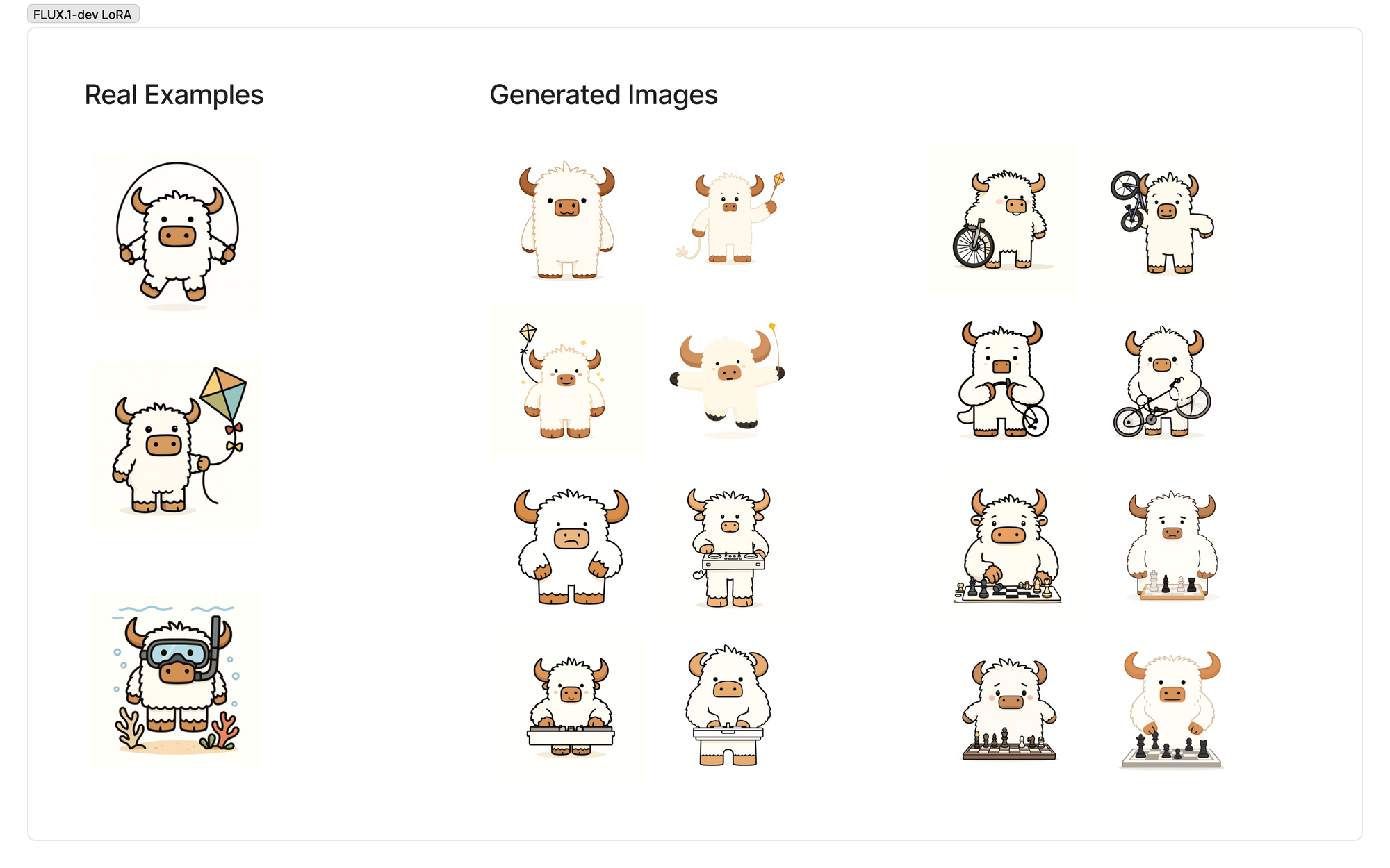
You can explore the whole training dataset here if you are interested.

A few weeks ago we did some exploration of fine-tuning PixArt and actually found this model much better for this style of vector graphic character.

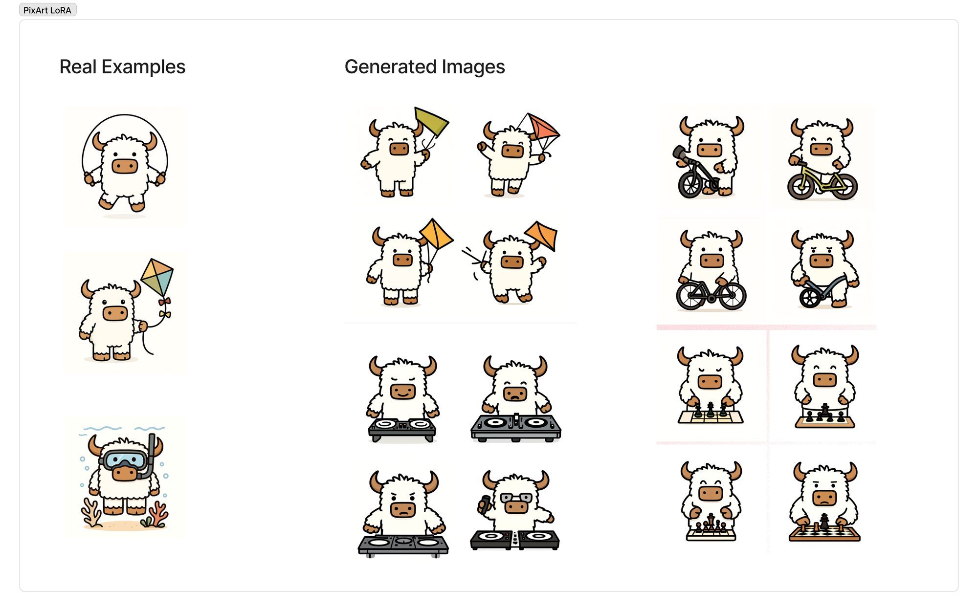
Our writeup and video on how to generate the synthetic data and train the model can be found here. Note: we did it on more Pixar-style Oxen in this post, but the recipe is the same.

The conclusion we came to is that FLUX is really good for photorealistic images, but may take some additional hyper parameter tuning to work well for simple vector graphics. PixArt nailed it right out of the gate, and was much faster to train since it is a smaller model.

🐂 Join the Herd!

If you enjoyed this post, feel free to join us live for Fine-Tuning Fridays! Each week we pick a model to fine-tune and compare the results on real world use cases. We post the live events on lu.ma/oxen.

We are also integrating zero-code fine-tuning into the Oxen.ai product. Feel free to sign up for a free account and test it out yourself. We give you access to the raw code, data and model weights so that you know exactly what is going on under the hood. Our goal is to make it as easy as possible to customize your models given your proprietary data.

Learn more here: